pacman::p_load(tidyverse, reshape2, ggthemes,
               ggdist, patchwork, ggridges,
               ggrepel, knitr, lubridate,
patchwork)Take-home Exercise 1 (Part 2): DataVis Makeover
1 Overview
In Take-home Exercise 1 (Part 1), we were tasked to produce two to three data visualisations using ggplot2 and its extensions to reveal the private residential market and sub-markets of Singapore for the 1st quarter of 2024. The data preparation was also processed by using the tidyverse family of packages. The exercise allowed us to explore factors such as Transacted Price ($) and Unit Price ($ PSM) in relation to Property Typeand Planning Region to list a few.
For this Take-home Exercise 1 (Part 2), the objective is to perform a makeover and improve on the original data visualisation from other peers. We will be critiquing one data visualisation in terms of its clarity and aesthetics. A sketch of the alternative design will be done up based on the data visualisation design principles (four quadrants of clarity and aesthetic) and finally a remake of the original design will be implemented.
2 Getting Started
2.1 Installing and loading the required libraries
- tidyverse: (i.e. readr, tidyr, dplyr, ggplot2) for performing data science tasks such as importing, tidying, and wrangling data, as well as creating graphics based on The Grammar of Graphics,
- reshape2 for transforming data between wide and long formats
- ggthemes: provides some extra themes, geoms, and scales for ‘ggplot2’.
- ggdist: a ggplot2 extension specially designed for visualising distribution and uncertainty
- patchwork: an R package for preparing composite figure created using ggplot2.
- ggridges: a ggplot2 extension specially designed for plotting ridgeline plots.
- ggrepel: an R package which provides geoms for ggplot2 to repel overlapping text labels.
- knitr: for building static html table to aid us in having a better view of tables
- lubridate: R package that makes it easier to work with dates and times.
- patchwork: an R package for preparing composite figure created using ggplot2.
The code chunk below uses p_load() function from pacman package to check if packages listed are already installed in the computer. The packages will be loaded if they are found to be installed. Otherwise, the function will proceed to install and load them into R environment.
2.2 Data Import and Wrangling
The subsequent code chunks utilises the read_csv function to import the five .csv data files from REALIS into the R environment. The data will also be labelled as such for identification:
- 2023Q1: ResidentialTransaction20240308160536
- 2023Q2: ResidentialTransaction20240308160736
- 2023Q3: ResidentialTransaction20240308161009
- 2023Q4: ResidentialTransaction20240308161109
- 2024Q1: ResidentialTransaction20240414220633
The code chunk below utilises the rename_with() function to change the column names accordingly using column_rename as an object.
column_rename <- function(orig_name) {
  # Add underscores to spaces
  gsub(" +", "_",
       # Remove special characters
       gsub("[^A-Z ]", "",
            # Convert to upper case and remove trailing spaces
            toupper(orig_name)) %>% trimws())
}
property_2023q1 <- read_csv('data/ResidentialTransaction20240308160536.csv') %>%
rename_with(column_rename)
kable(head(property_2023q1, n=5))| PROJECT_NAME | TRANSACTED_PRICE | AREA_SQFT | UNIT_PRICE_PSF | SALE_DATE | ADDRESS | TYPE_OF_SALE | TYPE_OF_AREA | AREA_SQM | UNIT_PRICE_PSM | NETT_PRICE | PROPERTY_TYPE | NUMBER_OF_UNITS | TENURE | COMPLETION_DATE | PURCHASER_ADDRESS_INDICATOR | POSTAL_CODE | POSTAL_DISTRICT | POSTAL_SECTOR | PLANNING_REGION | PLANNING_AREA |
|---|---|---|---|---|---|---|---|---|---|---|---|---|---|---|---|---|---|---|---|---|
| THE REEF AT KING’S DOCK | 2317000 | 882.65 | 2625 | 01 Jan 2023 | 12 HARBOURFRONT AVENUE #05-32 | New Sale | Strata | 82 | 28256 | - | Condominium | 1 | 99 yrs from 12/01/2021 | Uncompleted | HDB | 097996 | 04 | 09 | Central Region | Bukit Merah |
| URBAN TREASURES | 1823500 | 882.65 | 2066 | 02 Jan 2023 | 205 JALAN EUNOS #08-02 | New Sale | Strata | 82 | 22238 | - | Condominium | 1 | Freehold | Uncompleted | Private | 419535 | 14 | 41 | East Region | Bedok |
| NORTH GAIA | 1421112 | 1076.40 | 1320 | 02 Jan 2023 | 29 YISHUN CLOSE #08-10 | New Sale | Strata | 100 | 14211 | - | Executive Condominium | 1 | 99 yrs from 15/02/2021 | Uncompleted | HDB | 269343 | 27 | 26 | North Region | Yishun |
| NORTH GAIA | 1258112 | 1033.34 | 1218 | 02 Jan 2023 | 45 YISHUN CLOSE #07-42 | New Sale | Strata | 96 | 13105 | - | Executive Condominium | 1 | 99 yrs from 15/02/2021 | Uncompleted | HDB | 269294 | 27 | 26 | North Region | Yishun |
| PARC BOTANNIA | 1280000 | 871.88 | 1468 | 03 Jan 2023 | 12 FERNVALE STREET #06-16 | Resale | Strata | 81 | 15802 | - | Condominium | 1 | 99 yrs from 28/12/2016 | 2022 | HDB | 797391 | 28 | 79 | North East Region | Sengkang |
property_2023q2 <- read_csv('data/ResidentialTransaction20240308160736.csv') %>%
                  rename_with(column_rename)
kable(head(property_2023q1, n=5))| PROJECT_NAME | TRANSACTED_PRICE | AREA_SQFT | UNIT_PRICE_PSF | SALE_DATE | ADDRESS | TYPE_OF_SALE | TYPE_OF_AREA | AREA_SQM | UNIT_PRICE_PSM | NETT_PRICE | PROPERTY_TYPE | NUMBER_OF_UNITS | TENURE | COMPLETION_DATE | PURCHASER_ADDRESS_INDICATOR | POSTAL_CODE | POSTAL_DISTRICT | POSTAL_SECTOR | PLANNING_REGION | PLANNING_AREA |
|---|---|---|---|---|---|---|---|---|---|---|---|---|---|---|---|---|---|---|---|---|
| THE REEF AT KING’S DOCK | 2317000 | 882.65 | 2625 | 01 Jan 2023 | 12 HARBOURFRONT AVENUE #05-32 | New Sale | Strata | 82 | 28256 | - | Condominium | 1 | 99 yrs from 12/01/2021 | Uncompleted | HDB | 097996 | 04 | 09 | Central Region | Bukit Merah |
| URBAN TREASURES | 1823500 | 882.65 | 2066 | 02 Jan 2023 | 205 JALAN EUNOS #08-02 | New Sale | Strata | 82 | 22238 | - | Condominium | 1 | Freehold | Uncompleted | Private | 419535 | 14 | 41 | East Region | Bedok |
| NORTH GAIA | 1421112 | 1076.40 | 1320 | 02 Jan 2023 | 29 YISHUN CLOSE #08-10 | New Sale | Strata | 100 | 14211 | - | Executive Condominium | 1 | 99 yrs from 15/02/2021 | Uncompleted | HDB | 269343 | 27 | 26 | North Region | Yishun |
| NORTH GAIA | 1258112 | 1033.34 | 1218 | 02 Jan 2023 | 45 YISHUN CLOSE #07-42 | New Sale | Strata | 96 | 13105 | - | Executive Condominium | 1 | 99 yrs from 15/02/2021 | Uncompleted | HDB | 269294 | 27 | 26 | North Region | Yishun |
| PARC BOTANNIA | 1280000 | 871.88 | 1468 | 03 Jan 2023 | 12 FERNVALE STREET #06-16 | Resale | Strata | 81 | 15802 | - | Condominium | 1 | 99 yrs from 28/12/2016 | 2022 | HDB | 797391 | 28 | 79 | North East Region | Sengkang |
property_2023q3 <- read_csv('data/ResidentialTransaction20240308161009.csv') %>%
                  rename_with(column_rename)
kable(head(property_2023q1, n=5))| PROJECT_NAME | TRANSACTED_PRICE | AREA_SQFT | UNIT_PRICE_PSF | SALE_DATE | ADDRESS | TYPE_OF_SALE | TYPE_OF_AREA | AREA_SQM | UNIT_PRICE_PSM | NETT_PRICE | PROPERTY_TYPE | NUMBER_OF_UNITS | TENURE | COMPLETION_DATE | PURCHASER_ADDRESS_INDICATOR | POSTAL_CODE | POSTAL_DISTRICT | POSTAL_SECTOR | PLANNING_REGION | PLANNING_AREA |
|---|---|---|---|---|---|---|---|---|---|---|---|---|---|---|---|---|---|---|---|---|
| THE REEF AT KING’S DOCK | 2317000 | 882.65 | 2625 | 01 Jan 2023 | 12 HARBOURFRONT AVENUE #05-32 | New Sale | Strata | 82 | 28256 | - | Condominium | 1 | 99 yrs from 12/01/2021 | Uncompleted | HDB | 097996 | 04 | 09 | Central Region | Bukit Merah |
| URBAN TREASURES | 1823500 | 882.65 | 2066 | 02 Jan 2023 | 205 JALAN EUNOS #08-02 | New Sale | Strata | 82 | 22238 | - | Condominium | 1 | Freehold | Uncompleted | Private | 419535 | 14 | 41 | East Region | Bedok |
| NORTH GAIA | 1421112 | 1076.40 | 1320 | 02 Jan 2023 | 29 YISHUN CLOSE #08-10 | New Sale | Strata | 100 | 14211 | - | Executive Condominium | 1 | 99 yrs from 15/02/2021 | Uncompleted | HDB | 269343 | 27 | 26 | North Region | Yishun |
| NORTH GAIA | 1258112 | 1033.34 | 1218 | 02 Jan 2023 | 45 YISHUN CLOSE #07-42 | New Sale | Strata | 96 | 13105 | - | Executive Condominium | 1 | 99 yrs from 15/02/2021 | Uncompleted | HDB | 269294 | 27 | 26 | North Region | Yishun |
| PARC BOTANNIA | 1280000 | 871.88 | 1468 | 03 Jan 2023 | 12 FERNVALE STREET #06-16 | Resale | Strata | 81 | 15802 | - | Condominium | 1 | 99 yrs from 28/12/2016 | 2022 | HDB | 797391 | 28 | 79 | North East Region | Sengkang |
property_2023q4 <- read_csv('data/ResidentialTransaction20240308161109.csv') %>%
                  rename_with(column_rename)
kable(head(property_2023q1, n=5))| PROJECT_NAME | TRANSACTED_PRICE | AREA_SQFT | UNIT_PRICE_PSF | SALE_DATE | ADDRESS | TYPE_OF_SALE | TYPE_OF_AREA | AREA_SQM | UNIT_PRICE_PSM | NETT_PRICE | PROPERTY_TYPE | NUMBER_OF_UNITS | TENURE | COMPLETION_DATE | PURCHASER_ADDRESS_INDICATOR | POSTAL_CODE | POSTAL_DISTRICT | POSTAL_SECTOR | PLANNING_REGION | PLANNING_AREA |
|---|---|---|---|---|---|---|---|---|---|---|---|---|---|---|---|---|---|---|---|---|
| THE REEF AT KING’S DOCK | 2317000 | 882.65 | 2625 | 01 Jan 2023 | 12 HARBOURFRONT AVENUE #05-32 | New Sale | Strata | 82 | 28256 | - | Condominium | 1 | 99 yrs from 12/01/2021 | Uncompleted | HDB | 097996 | 04 | 09 | Central Region | Bukit Merah |
| URBAN TREASURES | 1823500 | 882.65 | 2066 | 02 Jan 2023 | 205 JALAN EUNOS #08-02 | New Sale | Strata | 82 | 22238 | - | Condominium | 1 | Freehold | Uncompleted | Private | 419535 | 14 | 41 | East Region | Bedok |
| NORTH GAIA | 1421112 | 1076.40 | 1320 | 02 Jan 2023 | 29 YISHUN CLOSE #08-10 | New Sale | Strata | 100 | 14211 | - | Executive Condominium | 1 | 99 yrs from 15/02/2021 | Uncompleted | HDB | 269343 | 27 | 26 | North Region | Yishun |
| NORTH GAIA | 1258112 | 1033.34 | 1218 | 02 Jan 2023 | 45 YISHUN CLOSE #07-42 | New Sale | Strata | 96 | 13105 | - | Executive Condominium | 1 | 99 yrs from 15/02/2021 | Uncompleted | HDB | 269294 | 27 | 26 | North Region | Yishun |
| PARC BOTANNIA | 1280000 | 871.88 | 1468 | 03 Jan 2023 | 12 FERNVALE STREET #06-16 | Resale | Strata | 81 | 15802 | - | Condominium | 1 | 99 yrs from 28/12/2016 | 2022 | HDB | 797391 | 28 | 79 | North East Region | Sengkang |
property_2024q1 <- read_csv('data/ResidentialTransaction20240414220633.csv') %>%
                  rename_with(column_rename)
kable(head(property_2023q1, n=5))| PROJECT_NAME | TRANSACTED_PRICE | AREA_SQFT | UNIT_PRICE_PSF | SALE_DATE | ADDRESS | TYPE_OF_SALE | TYPE_OF_AREA | AREA_SQM | UNIT_PRICE_PSM | NETT_PRICE | PROPERTY_TYPE | NUMBER_OF_UNITS | TENURE | COMPLETION_DATE | PURCHASER_ADDRESS_INDICATOR | POSTAL_CODE | POSTAL_DISTRICT | POSTAL_SECTOR | PLANNING_REGION | PLANNING_AREA |
|---|---|---|---|---|---|---|---|---|---|---|---|---|---|---|---|---|---|---|---|---|
| THE REEF AT KING’S DOCK | 2317000 | 882.65 | 2625 | 01 Jan 2023 | 12 HARBOURFRONT AVENUE #05-32 | New Sale | Strata | 82 | 28256 | - | Condominium | 1 | 99 yrs from 12/01/2021 | Uncompleted | HDB | 097996 | 04 | 09 | Central Region | Bukit Merah |
| URBAN TREASURES | 1823500 | 882.65 | 2066 | 02 Jan 2023 | 205 JALAN EUNOS #08-02 | New Sale | Strata | 82 | 22238 | - | Condominium | 1 | Freehold | Uncompleted | Private | 419535 | 14 | 41 | East Region | Bedok |
| NORTH GAIA | 1421112 | 1076.40 | 1320 | 02 Jan 2023 | 29 YISHUN CLOSE #08-10 | New Sale | Strata | 100 | 14211 | - | Executive Condominium | 1 | 99 yrs from 15/02/2021 | Uncompleted | HDB | 269343 | 27 | 26 | North Region | Yishun |
| NORTH GAIA | 1258112 | 1033.34 | 1218 | 02 Jan 2023 | 45 YISHUN CLOSE #07-42 | New Sale | Strata | 96 | 13105 | - | Executive Condominium | 1 | 99 yrs from 15/02/2021 | Uncompleted | HDB | 269294 | 27 | 26 | North Region | Yishun |
| PARC BOTANNIA | 1280000 | 871.88 | 1468 | 03 Jan 2023 | 12 FERNVALE STREET #06-16 | Resale | Strata | 81 | 15802 | - | Condominium | 1 | 99 yrs from 28/12/2016 | 2022 | HDB | 797391 | 28 | 79 | North East Region | Sengkang |
The code chunk below glimpse() will provide us with an overview of the data.
glimpse(property_2023q1)Rows: 4,722
Columns: 21
$ PROJECT_NAME <chr> "THE REEF AT KING'S DOCK", "URBAN TREASURE…
$ TRANSACTED_PRICE <dbl> 2317000, 1823500, 1421112, 1258112, 128000…
$ AREA_SQFT <dbl> 882.65, 882.65, 1076.40, 1033.34, 871.88, …
$ UNIT_PRICE_PSF <dbl> 2625, 2066, 1320, 1218, 1468, 1767, 1095, …
$ SALE_DATE <chr> "01 Jan 2023", "02 Jan 2023", "02 Jan 2023…
$ ADDRESS <chr> "12 HARBOURFRONT AVENUE #05-32", "205 JALA…
$ TYPE_OF_SALE <chr> "New Sale", "New Sale", "New Sale", "New S…
$ TYPE_OF_AREA <chr> "Strata", "Strata", "Strata", "Strata", "S…
$ AREA_SQM <dbl> 82.0, 82.0, 100.0, 96.0, 81.0, 308.7, 420.…
$ UNIT_PRICE_PSM <dbl> 28256, 22238, 14211, 13105, 15802, 19015, …
$ NETT_PRICE <chr> "-", "-", "-", "-", "-", "-", "-", "-", "-…
$ PROPERTY_TYPE <chr> "Condominium", "Condominium", "Executive C…
$ NUMBER_OF_UNITS <dbl> 1, 1, 1, 1, 1, 1, 1, 1, 1, 1, 1, 1, 1, 1, …
$ TENURE <chr> "99 yrs from 12/01/2021", "Freehold", "99 …
$ COMPLETION_DATE <chr> "Uncompleted", "Uncompleted", "Uncompleted…
$ PURCHASER_ADDRESS_INDICATOR <chr> "HDB", "Private", "HDB", "HDB", "HDB", "Pr…
$ POSTAL_CODE <chr> "097996", "419535", "269343", "269294", "7…
$ POSTAL_DISTRICT <chr> "04", "14", "27", "27", "28", "19", "10", …
$ POSTAL_SECTOR <chr> "09", "41", "26", "26", "79", "54", "27", …
$ PLANNING_REGION <chr> "Central Region", "East Region", "North Re…
$ PLANNING_AREA <chr> "Bukit Merah", "Bedok", "Yishun", "Yishun"…glimpse(property_2023q2)Rows: 6,125
Columns: 21
$ PROJECT_NAME <chr> "THE GAZANIA", "THE GAZANIA", "ONE PEARL B…
$ TRANSACTED_PRICE <dbl> 1528000, 1938000, 2051000, 1850700, 202150…
$ AREA_SQFT <dbl> 678.13, 958.00, 699.66, 882.65, 699.66, 78…
$ UNIT_PRICE_PSF <dbl> 2253, 2023, 2931, 2097, 2889, 2339, 3560, …
$ SALE_DATE <chr> "01 Apr 2023", "01 Apr 2023", "01 Apr 2023…
$ ADDRESS <chr> "15 HOW SUN DRIVE #02-31", "7 HOW SUN DRIV…
$ TYPE_OF_SALE <chr> "New Sale", "New Sale", "New Sale", "New S…
$ TYPE_OF_AREA <chr> "Strata", "Strata", "Strata", "Strata", "S…
$ AREA_SQM <dbl> 63, 89, 65, 82, 65, 73, 191, 46, 62, 93, 8…
$ UNIT_PRICE_PSM <dbl> 24254, 21775, 31554, 22570, 31100, 25178, …
$ NETT_PRICE <chr> "-", "-", "-", "-", "-", "-", "-", "-", "-…
$ PROPERTY_TYPE <chr> "Condominium", "Condominium", "Apartment",…
$ NUMBER_OF_UNITS <dbl> 1, 1, 1, 1, 1, 1, 1, 1, 1, 1, 1, 1, 1, 1, …
$ TENURE <chr> "Freehold", "Freehold", "99 yrs from 01/03…
$ COMPLETION_DATE <chr> "2022", "2022", "Uncompleted", "Uncomplete…
$ PURCHASER_ADDRESS_INDICATOR <chr> "N.A", "Private", "Private", "HDB", "Priva…
$ POSTAL_CODE <chr> "538545", "538530", "169016", "419535", "2…
$ POSTAL_DISTRICT <chr> "19", "19", "03", "14", "10", "10", "09", …
$ POSTAL_SECTOR <chr> "53", "53", "16", "41", "27", "26", "22", …
$ PLANNING_REGION <chr> "North East Region", "North East Region", …
$ PLANNING_AREA <chr> "Serangoon", "Serangoon", "Outram", "Bedok…glimpse(property_2023q3)Rows: 6,206
Columns: 21
$ PROJECT_NAME <chr> "MYRA", "NORTH GAIA", "NORTH GAIA", "NORTH…
$ TRANSACTED_PRICE <dbl> 1658000, 1449000, 1365000, 1231000, 127200…
$ AREA_SQFT <dbl> 667.37, 1076.40, 1076.40, 958.00, 1001.05,…
$ UNIT_PRICE_PSF <dbl> 2484, 1346, 1268, 1285, 1271, 2062, 1465, …
$ SALE_DATE <chr> "01 Jul 2023", "01 Jul 2023", "01 Jul 2023…
$ ADDRESS <chr> "9 MEYAPPA CHETTIAR ROAD #02-07", "27 YISH…
$ TYPE_OF_SALE <chr> "New Sale", "New Sale", "New Sale", "New S…
$ TYPE_OF_AREA <chr> "Strata", "Strata", "Strata", "Strata", "S…
$ AREA_SQM <dbl> 62, 100, 100, 89, 93, 156, 86, 86, 86, 86,…
$ UNIT_PRICE_PSM <dbl> 26742, 14490, 13650, 13831, 13677, 22192, …
$ NETT_PRICE <chr> "-", "-", "-", "-", "-", "-", "-", "-", "-…
$ PROPERTY_TYPE <chr> "Apartment", "Executive Condominium", "Exe…
$ NUMBER_OF_UNITS <dbl> 1, 1, 1, 1, 1, 1, 1, 1, 1, 1, 1, 1, 1, 1, …
$ TENURE <chr> "Freehold", "99 yrs from 15/02/2021", "99 …
$ COMPLETION_DATE <chr> "Uncompleted", "Uncompleted", "Uncompleted…
$ PURCHASER_ADDRESS_INDICATOR <chr> "N.A", "HDB", "HDB", "HDB", "HDB", "Privat…
$ POSTAL_CODE <chr> "358456", "769342", "769342", "769299", "7…
$ POSTAL_DISTRICT <chr> "13", "27", "27", "27", "27", "08", "18", …
$ POSTAL_SECTOR <chr> "35", "76", "76", "76", "76", "21", "52", …
$ PLANNING_REGION <chr> "Central Region", "North Region", "North R…
$ PLANNING_AREA <chr> "Toa Payoh", "Yishun", "Yishun", "Yishun",…glimpse(property_2023q4)Rows: 4,851
Columns: 21
$ PROJECT_NAME <chr> "LEEDON GREEN", "LIV @ MB", "MORI", "THE A…
$ TRANSACTED_PRICE <dbl> 1749000, 3148740, 2422337, 1330000, 223700…
$ AREA_SQFT <dbl> 538.20, 1453.14, 1259.39, 721.19, 1130.22,…
$ UNIT_PRICE_PSF <dbl> 3250, 2167, 1923, 1844, 1979, 2111, 2131, …
$ SALE_DATE <chr> "01 Oct 2023", "01 Oct 2023", "01 Oct 2023…
$ ADDRESS <chr> "26 LEEDON HEIGHTS #11-08", "114A ARTHUR R…
$ TYPE_OF_SALE <chr> "New Sale", "New Sale", "New Sale", "New S…
$ TYPE_OF_AREA <chr> "Strata", "Strata", "Strata", "Strata", "S…
$ AREA_SQM <dbl> 50.0, 135.0, 117.0, 67.0, 105.0, 55.0, 126…
$ UNIT_PRICE_PSM <dbl> 34980, 23324, 20704, 19851, 21305, 22725, …
$ NETT_PRICE <chr> "-", "-", "-", "-", "-", "-", "-", "-", "-…
$ PROPERTY_TYPE <chr> "Condominium", "Condominium", "Apartment",…
$ NUMBER_OF_UNITS <dbl> 1, 1, 1, 1, 1, 1, 1, 1, 1, 1, 1, 1, 1, 1, …
$ TENURE <chr> "Freehold", "99 yrs from 23/11/2021", "Fre…
$ COMPLETION_DATE <chr> "Uncompleted", "Uncompleted", "Uncompleted…
$ PURCHASER_ADDRESS_INDICATOR <chr> "Private", "Private", "Private", "Private"…
$ POSTAL_CODE <chr> "266221", "439826", "399738", "668159", "7…
$ POSTAL_DISTRICT <chr> "10", "15", "14", "23", "26", "22", "26", …
$ POSTAL_SECTOR <chr> "26", "43", "39", "66", "78", "61", "78", …
$ PLANNING_REGION <chr> "Central Region", "Central Region", "Centr…
$ PLANNING_AREA <chr> "Bukit Timah", "Marine Parade", "Geylang",…glimpse(property_2024q1)Rows: 4,902
Columns: 21
$ PROJECT_NAME <chr> "THE LANDMARK", "POLLEN COLLECTION", "SKY …
$ TRANSACTED_PRICE <dbl> 2726888, 3850000, 2346000, 2190000, 195400…
$ AREA_SQFT <dbl> 1076.40, 1808.35, 1087.16, 807.30, 796.54,…
$ UNIT_PRICE_PSF <dbl> 2533, 2129, 2158, 2713, 2453, 2577, 838, 1…
$ SALE_DATE <chr> "01 Jan 2024", "01 Jan 2024", "01 Jan 2024…
$ ADDRESS <chr> "173 CHIN SWEE ROAD #22-11", "34 POLLEN PL…
$ TYPE_OF_SALE <chr> "New Sale", "New Sale", "New Sale", "New S…
$ TYPE_OF_AREA <chr> "Strata", "Land", "Strata", "Strata", "Str…
$ AREA_SQM <dbl> 100.0, 168.0, 101.0, 75.0, 74.0, 123.0, 32…
$ UNIT_PRICE_PSM <dbl> 27269, 22917, 23228, 29200, 26405, 27741, …
$ NETT_PRICE <chr> "-", "-", "-", "-", "-", "-", "-", "-", "-…
$ PROPERTY_TYPE <chr> "Condominium", "Terrace House", "Apartment…
$ NUMBER_OF_UNITS <dbl> 1, 1, 1, 1, 1, 1, 1, 1, 1, 1, 1, 1, 1, 1, …
$ TENURE <chr> "99 yrs from 28/08/2020", "99 yrs from 09/…
$ COMPLETION_DATE <chr> "Uncompleted", "Uncompleted", "Uncompleted…
$ PURCHASER_ADDRESS_INDICATOR <chr> "Private", "N.A", "HDB", "N.A", "Private",…
$ POSTAL_CODE <chr> "169878", "807233", "469657", "118992", "5…
$ POSTAL_DISTRICT <chr> "03", "28", "16", "05", "21", "21", "28", …
$ POSTAL_SECTOR <chr> "16", "80", "46", "11", "59", "58", "79", …
$ PLANNING_REGION <chr> "Central Region", "North East Region", "Ea…
$ PLANNING_AREA <chr> "Outram", "Serangoon", "Bedok", "Queenstow…Data Wrangling
property_2023q1 <- property_2023q1 %>%
  mutate(
    QUARTER="2023Q1",
    MONTH_YEAR=format(dmy(SALE_DATE), "%b-%y")
  )
property_2023q2 <- property_2023q2 %>%
  mutate(
    QUARTER="2023Q2",
    MONTH_YEAR=format(dmy(SALE_DATE), "%b-%y")
  )
property_2023q3 <- property_2023q3 %>%
  mutate(
    QUARTER="2023Q3",
    MONTH_YEAR=format(dmy(SALE_DATE), "%b-%y")
  )
property_2023q4 <- property_2023q4 %>%
  mutate(
    QUARTER="2023Q4",
    MONTH_YEAR=format(dmy(SALE_DATE), "%b-%y")
  )
property_2024q1 <- property_2024q1 %>%
  mutate(
    QUARTER="2024Q1",
    MONTH_YEAR=format(dmy(SALE_DATE), "%b-%y")
  )
realis <- property_2023q1 %>%
rbind(property_2023q2) %>%
rbind(property_2023q3) %>%
rbind(property_2023q4) %>%
rbind(property_2024q1)
kable(head(realis, n=10))| PROJECT_NAME | TRANSACTED_PRICE | AREA_SQFT | UNIT_PRICE_PSF | SALE_DATE | ADDRESS | TYPE_OF_SALE | TYPE_OF_AREA | AREA_SQM | UNIT_PRICE_PSM | NETT_PRICE | PROPERTY_TYPE | NUMBER_OF_UNITS | TENURE | COMPLETION_DATE | PURCHASER_ADDRESS_INDICATOR | POSTAL_CODE | POSTAL_DISTRICT | POSTAL_SECTOR | PLANNING_REGION | PLANNING_AREA | QUARTER | MONTH_YEAR |
|---|---|---|---|---|---|---|---|---|---|---|---|---|---|---|---|---|---|---|---|---|---|---|
| THE REEF AT KING’S DOCK | 2317000 | 882.65 | 2625 | 01 Jan 2023 | 12 HARBOURFRONT AVENUE #05-32 | New Sale | Strata | 82.0 | 28256 | - | Condominium | 1 | 99 yrs from 12/01/2021 | Uncompleted | HDB | 097996 | 04 | 09 | Central Region | Bukit Merah | 2023Q1 | Jan-23 |
| URBAN TREASURES | 1823500 | 882.65 | 2066 | 02 Jan 2023 | 205 JALAN EUNOS #08-02 | New Sale | Strata | 82.0 | 22238 | - | Condominium | 1 | Freehold | Uncompleted | Private | 419535 | 14 | 41 | East Region | Bedok | 2023Q1 | Jan-23 |
| NORTH GAIA | 1421112 | 1076.40 | 1320 | 02 Jan 2023 | 29 YISHUN CLOSE #08-10 | New Sale | Strata | 100.0 | 14211 | - | Executive Condominium | 1 | 99 yrs from 15/02/2021 | Uncompleted | HDB | 269343 | 27 | 26 | North Region | Yishun | 2023Q1 | Jan-23 |
| NORTH GAIA | 1258112 | 1033.34 | 1218 | 02 Jan 2023 | 45 YISHUN CLOSE #07-42 | New Sale | Strata | 96.0 | 13105 | - | Executive Condominium | 1 | 99 yrs from 15/02/2021 | Uncompleted | HDB | 269294 | 27 | 26 | North Region | Yishun | 2023Q1 | Jan-23 |
| PARC BOTANNIA | 1280000 | 871.88 | 1468 | 03 Jan 2023 | 12 FERNVALE STREET #06-16 | Resale | Strata | 81.0 | 15802 | - | Condominium | 1 | 99 yrs from 28/12/2016 | 2022 | HDB | 797391 | 28 | 79 | North East Region | Sengkang | 2023Q1 | Jan-23 |
| NANYANG PARK | 5870000 | 3322.85 | 1767 | 03 Jan 2023 | 72 JALAN LIMBOK | Resale | Land | 308.7 | 19015 | - | Terrace House | 1 | 999 yrs from 14/02/1881 | - | Private | 548742 | 19 | 54 | North East Region | Hougang | 2023Q1 | Jan-23 |
| PALMS @ SIXTH AVENUE | 4950000 | 4520.88 | 1095 | 03 Jan 2023 | 231 SIXTH AVENUE | Resale | Strata | 420.0 | 11786 | - | Semi-Detached House | 1 | Freehold | 2015 | Private | 275780 | 10 | 27 | Central Region | Bukit Timah | 2023Q1 | Jan-23 |
| N.A. | 3260000 | 1555.40 | 2096 | 03 Jan 2023 | 19 TENG TONG ROAD | Resale | Land | 144.5 | 22561 | - | Terrace House | 1 | Freehold | 1941 | Private | 423510 | 15 | 42 | Central Region | Marine Parade | 2023Q1 | Jan-23 |
| WHISTLER GRAND | 850000 | 441.32 | 1926 | 03 Jan 2023 | 107 WEST COAST VALE #30-04 | Sub Sale | Strata | 41.0 | 20732 | - | Apartment | 1 | 99 yrs from 07/05/2018 | 2022 | HDB | 126751 | 05 | 12 | West Region | Clementi | 2023Q1 | Jan-23 |
| NORTHOAKS | 1268000 | 1603.84 | 791 | 03 Jan 2023 | 30 WOODLANDS CRESCENT #01-11 | Resale | Strata | 149.0 | 8510 | - | Executive Condominium | 1 | 99 yrs from 16/12/1997 | 2000 | HDB | 738086 | 25 | 73 | North Region | Woodlands | 2023Q1 | Jan-23 |
After adding the QUARTER columns, there are now 22 variables in the dataframe. However, for this exercise not all of them are necessary to carry out the analysis. We shall filter out the necessary columns and drop the rest for efficiency.
realis <-
  realis %>% select(
    c(
      QUARTER,
      MONTH_YEAR,
      PROPERTY_TYPE,
      PLANNING_REGION,
      PLANNING_AREA,
      TRANSACTED_PRICE,
      AREA_SQFT,
      UNIT_PRICE_PSF,
      SALE_DATE
    )
  )
glimpse(realis) #Overview of transformed data
Rows: 26,806
Columns: 9
$ QUARTER <chr> "2023Q1", "2023Q1", "2023Q1", "2023Q1", "2023Q1", "20…
$ MONTH_YEAR <chr> "Jan-23", "Jan-23", "Jan-23", "Jan-23", "Jan-23", "Ja…
$ PROPERTY_TYPE <chr> "Condominium", "Condominium", "Executive Condominium"…
$ PLANNING_REGION <chr> "Central Region", "East Region", "North Region", "Nor…
$ PLANNING_AREA <chr> "Bukit Merah", "Bedok", "Yishun", "Yishun", "Sengkang…
$ TRANSACTED_PRICE <dbl> 2317000, 1823500, 1421112, 1258112, 1280000, 5870000,…
$ AREA_SQFT <dbl> 882.65, 882.65, 1076.40, 1033.34, 871.88, 3322.85, 45…
$ UNIT_PRICE_PSF <dbl> 2625, 2066, 1320, 1218, 1468, 1767, 1095, 2096, 1926,…
$ SALE_DATE <chr> "01 Jan 2023", "02 Jan 2023", "02 Jan 2023", "02 Jan …Upon using glimpse(), it can be observed that there are 9 variables relevant to our data viz makeover.
3 Data Visualisation Makeover
In this section, we will proceed with a makeover of a peer’s data visualisation and building an improved version. Shown below is the plot of our peer’s plot.
The author stated:
As we mentioned about the individual market is focus on the apartment and condominium above, and we know the distribution of total property, what about the first quarter unit price of these two popular goods?
Upon examination of the violin plots, a clear disparity emerges between the average unit prices of condominiums and apartments, standing at approximately $1,500 and $2,000, respectively, for the period spanning January to March. Noteworthy is the discernible uptick in both unit price and transaction volume from January to March 2024. Despite an overall reduction in total transactions vis-a-vis the preceding year, there is an unmistakable trend towards growth within specific sub-markets, suggesting an increasing inclination towards higher-value properties
filtered_data <- combined_data %>%
  mutate(Sale_Date = dmy(`Sale Date`)) %>%
  filter((year(Sale_Date) == 2023 &
          month(Sale_Date) %in% 1:12) |
         (year(Sale_Date) == 2024 &
          month(Sale_Date) %in% 1:3)) %>%
  mutate(Quarter_Sale_Data = case_when(
    between(Sale_Date, as.Date("2023-01-01"), as.Date("2023-03-31")) ~ "Q1_2023",
    between(Sale_Date, as.Date("2023-04-01"), as.Date("2023-06-30")) ~ "Q2_2023",
    between(Sale_Date, as.Date("2023-07-01"), as.Date("2023-09-30")) ~ "Q3_2023",
    between(Sale_Date, as.Date("2023-10-01"), as.Date("2023-12-31")) ~ "Q4_2023",
    between(Sale_Date, as.Date("2024-01-01"), as.Date("2024-03-31")) ~ "Q1_2024",
    TRUE ~ NA_character_
  )) %>%
  filter(!is.na(Quarter_Sale_Data)) %>%
  mutate(Month_Sale_Data = paste0(year(Sale_Date), "-", month(Sale_Date)))

filtered_data <- filtered_data %>%
  filter(`Property Type` %in% c("Apartment", "Condominium"))

ggplot(filtered_data, aes(x = Month_Sale_Data, y = `Unit Price ($ PSF)`, color = `Property Type`)) +
  geom_violin() +
  geom_point(position = "jitter",
             size = 0.1) +
  labs(title = "Unit Price per Square Foot for Apartments and Condominiums",
       x = "Month",
       y = "Unit Price ($ PSF)") +
  theme_light(base_size = 6) +
  xlim(c("2024-1","2024-2","2024-3"))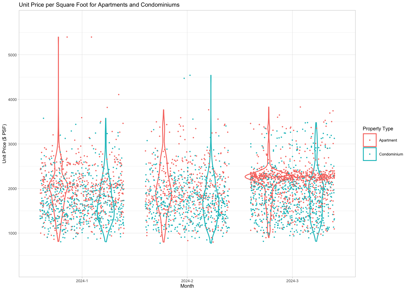
ggplot(filtered_data, aes(x = Month_Sale_Data, y = `Unit Price ($ PSF)`, color = `Property Type`)) +
  geom_violin() +
  geom_point(position = "jitter",
             size = 0.1) +
  labs(title = "Unit Price per Square Foot for Apartments and Condominiums",
       x = "Month",
       y = "Unit Price ($ PSF)") +
  theme_light(base_size = 6) +
  xlim(c("2023-1","2023-2","2023-3"))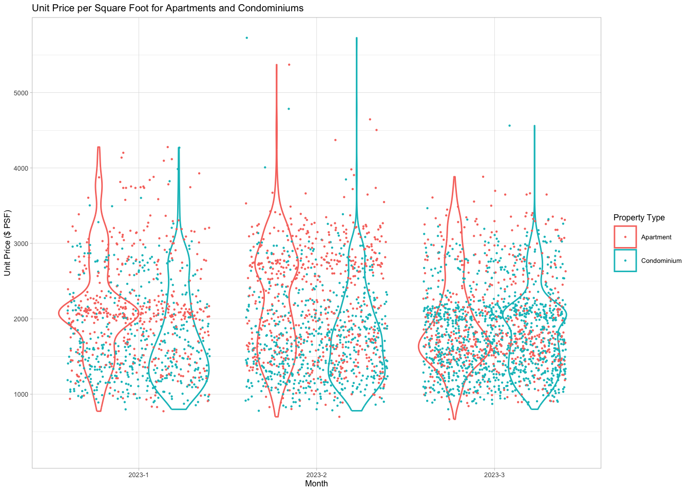
3.1 Observations: Clarity and Aesthetics
Clarity
The use of a violin plot overlaid with scatter plot points helps illustrate the distribution of prices per square foot for both apartments and condominiums across different months.
The red (apartment) and teal (condominium) color distinction or scatterplot is generally clear, but there’s significant overlap in data points, which may confuse the viewer about the exact differences in price distributions between these property types. This might also affect the ease of reading and understanding by audiences from the general public.
Aesthetics
The main title while clear could be centralised for easier readability.
The plot successfully uses colour to differentiate between the two types of properties. The choice of colors is visually distinct, which is helpful for quick differentiation.
However, the presence of outliers, particularly those extreme values shown as vertical lines extending from the main bodies of the violins, can confuse readers from the overall trends from the plot.
3.2 Sketch of alternative design
 Improvements based on the above points mentioned earlier:
Main title which was centred to give improved balanced to the plot layout.
Combine each different selected property type into each portion of the chart, sharing the same y-axis to reveal the distribution among different property types simultaneously.
Added additional pointers and/or labels to highlight summary statistic values such as Mean, Median and IQR.
Address the issue of outliers in the plot for this case I have chosen to highlight the outliers to enable readers to be aware and take note of them since they were still actual property transactions.
Use widely different colours to differentiate between the variables for better visual distinction.
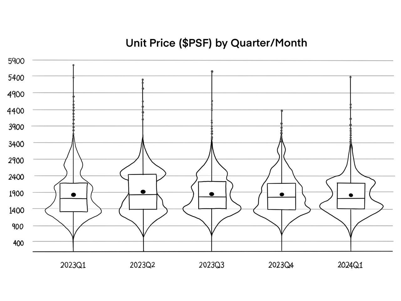
3.3 Remake of Original Design
1st iteration
Derived from the sketch ideation, this plot shows Unit Price ($ PSF) by Quarter as a start.
ggplot(data= realis,
       aes(x= QUARTER, y= UNIT_PRICE_PSF, color = QUARTER)) +
  geom_violin(aes(fill = QUARTER), size = 0.6, alpha = 0.3, linewidth = 0) +
  geom_boxplot(width= 0.4, outlier.colour = "grey20", outlier.size = 1,
               outlier.alpha = 0.3) +
  stat_summary(geom = "point",
               fun.y="mean",
               colour ="black",
               size=2) +
  coord_cartesian(ylim = c(400,6000)) +
  scale_color_manual(values=c("#c73824", "#0477bf", "#9E9E9E", "#0CDBBC", "#0437bf")) +
  theme_economist() +
  labs(title="Unit Price ($PSF) by Quarter") +
  scale_y_continuous(breaks = seq(400, 6000, by = 500)) +
  theme(axis.title.x = element_blank(),
        axis.title.y = element_blank(),
        plot.title=element_text(size= 12, hjust= 0.5),
        axis.text = element_text(size= 10),
        legend.position = "none")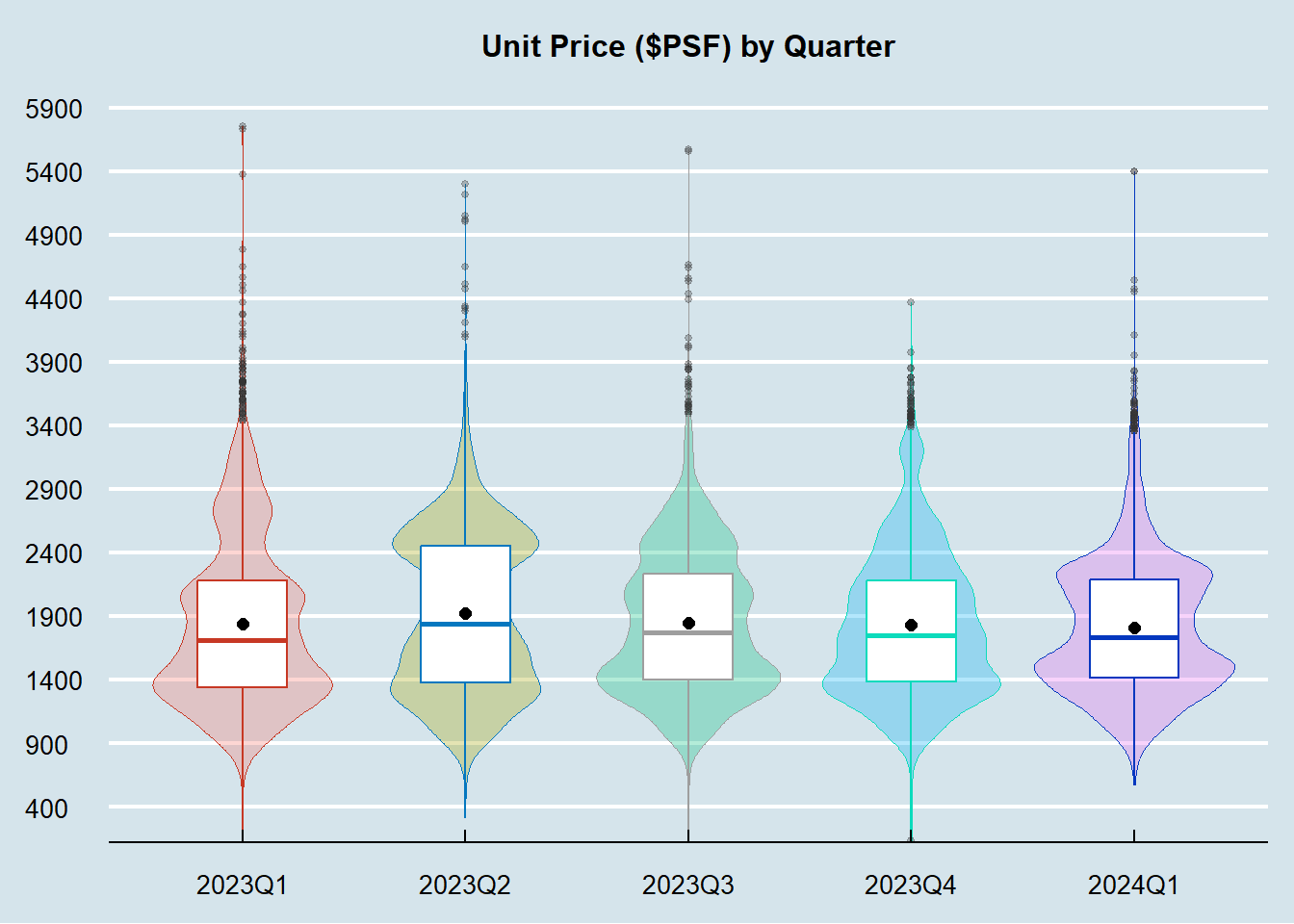
2nd iteration (Filtering of variables)
To accommodate to the peer’s selection of selected property type
filtered_data <- realis %>%
  filter(PROPERTY_TYPE %in% c("Apartment", "Condominium"),
         QUARTER %in% c("2023Q1", "2024Q1"))

ggplot(data= filtered_data,
       aes(x= QUARTER, y= UNIT_PRICE_PSF, color = QUARTER)) +
  geom_violin(aes(fill = QUARTER), size = 0.6, alpha = 0.3, linewidth = 0) +
  geom_boxplot(width= 0.4, outlier.colour = "grey20", outlier.size = 1,
               outlier.alpha = 0.3) +
  stat_summary(geom = "point",
               fun.y="mean",
               colour ="black",
               size=2) +
  coord_cartesian(ylim = c(400,6000)) +
  scale_color_manual(values=c("#c73824", "#0477bf", "#9E9E9E", "#0CDBBC", "#0437bf")) +
  theme_economist() +
  labs(title="Unit Price ($PSF) by Quarter") +
  scale_y_continuous(breaks = seq(400, 6000, by = 500)) +
  theme(axis.title.x = element_blank(),
        axis.title.y = element_blank(),
        plot.title=element_text(size= 12, hjust= 0.5),
        axis.text = element_text(size= 10),
        legend.position = "none") +
  facet_wrap(~PROPERTY_TYPE)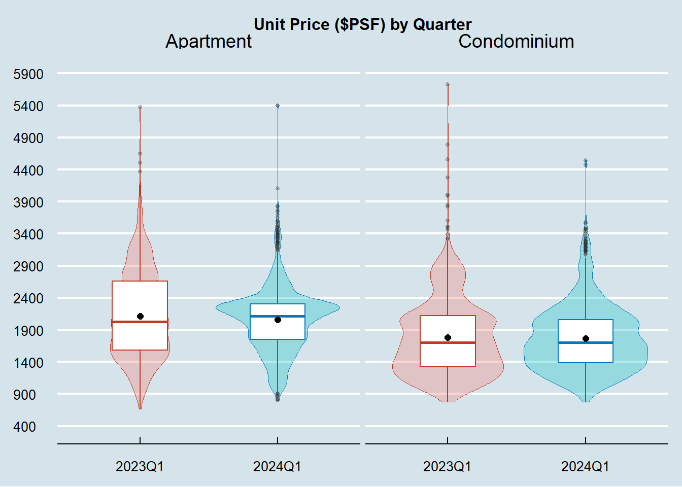
3rd iteration (Filtering of variables)
To accommodate to the peer’s selection of time period (Month)
filtered_data <- realis %>%
  filter(PROPERTY_TYPE %in% c("Apartment", "Condominium"),
         MONTH_YEAR %in% c("Jan-23", "Feb-23", "Mar-23")) %>%
  mutate(MONTH_YEAR = factor(MONTH_YEAR, levels = c("Jan-23", "Feb-23", "Mar-23")))

ggplot(data= filtered_data,
       aes(x= MONTH_YEAR, y= UNIT_PRICE_PSF, color = MONTH_YEAR)) +
  geom_violin(aes(fill = MONTH_YEAR), size = 0.6, alpha = 0.3, linewidth = 0) +
  geom_boxplot(width= 0.4, outlier.colour = "grey20", outlier.size = 1,
               outlier.alpha = 0.3) +
  stat_summary(geom = "point",
               fun.y="mean",
               colour ="black",
               size=2) +
  coord_cartesian(ylim = c(400,6000)) +
  scale_color_manual(values=c("#c73824", "#0477bf", "#9E9E9E", "#0CDBBC", "#0437bf")) +
  theme_economist() +
  labs(title="Unit Price ($PSF) by Month") +
  scale_y_continuous(breaks = seq(400, 6000, by = 500)) +
  theme(axis.title.x = element_blank(),
        axis.title.y = element_blank(),
        plot.title=element_text(size= 12, hjust= 0.5),
        axis.text = element_text(size= 10),
        legend.position = "none") +
  facet_wrap(~PROPERTY_TYPE)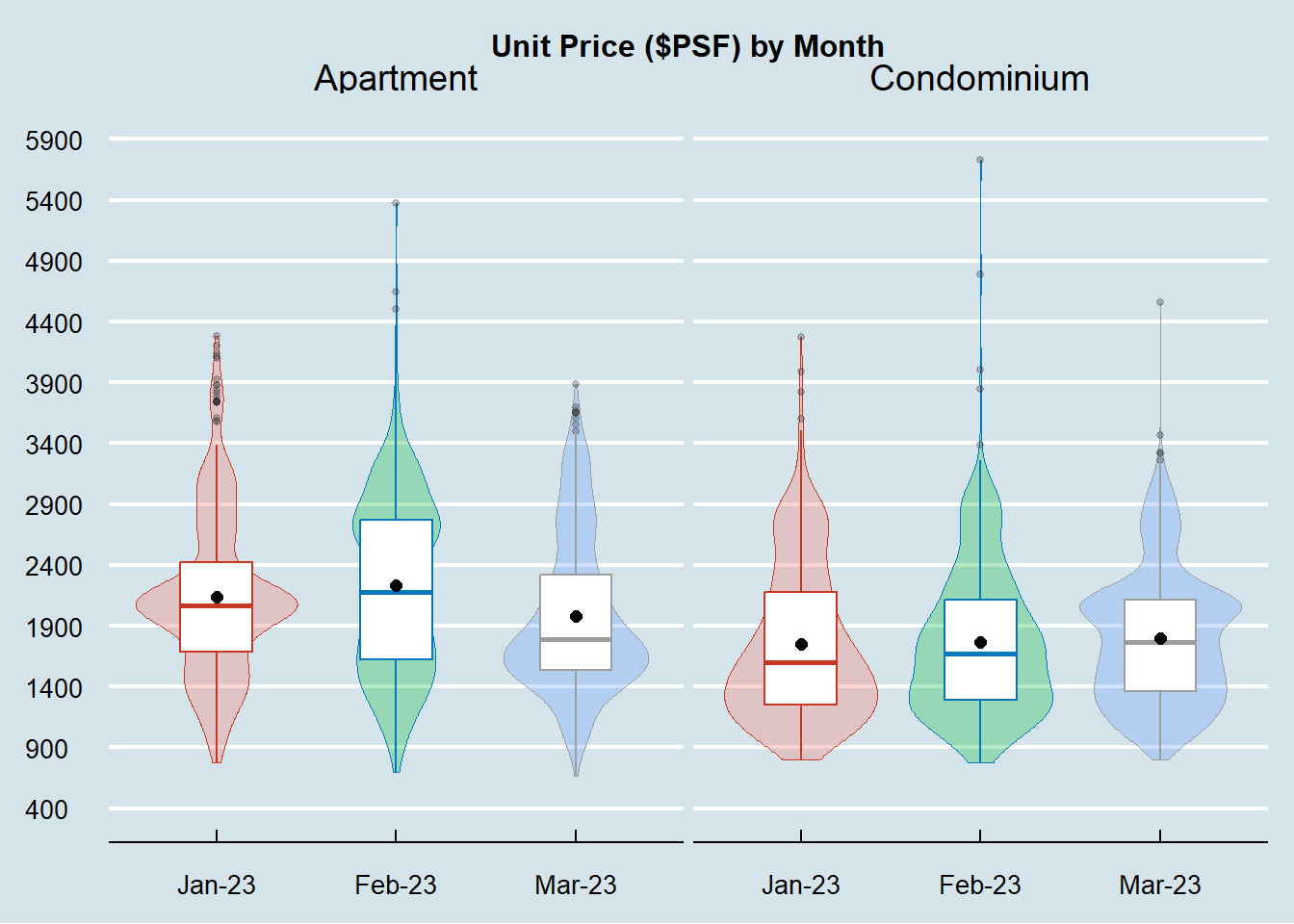
4th iteration (Addition of Summary Statistics)
For Year 2023
# Filter and order the data as before
filtered_data <- realis %>%
  filter(PROPERTY_TYPE %in% c("Apartment", "Condominium"),
         MONTH_YEAR %in% c("Jan-23", "Feb-23", "Mar-23")) %>%
  mutate(MONTH_YEAR = factor(MONTH_YEAR, levels = c("Jan-23", "Feb-23", "Mar-23")))

# Calculate summary statistics for annotations
stats_data <- filtered_data %>%
  group_by(MONTH_YEAR, PROPERTY_TYPE) %>%
  summarise(
    Mean = mean(UNIT_PRICE_PSF),
    Median = median(UNIT_PRICE_PSF),
    IQR = IQR(UNIT_PRICE_PSF),
    .groups = 'drop'
  )

# Generate the violin plot with statistical annotations
plot1 <- ggplot(data = filtered_data,
       aes(x = MONTH_YEAR, y = UNIT_PRICE_PSF, color = MONTH_YEAR)) +
  geom_violin(aes(fill = MONTH_YEAR), size = 0.6, alpha = 0.3, linewidth = 0) +
  geom_boxplot(width = 0.4, outlier.colour = "grey20", outlier.size = 1,
               outlier.alpha = 0.3) +
  stat_summary(geom = "point",
               fun.y="mean",
               colour ="black",
               size=2) +
  geom_text(data = stats_data, aes(label = sprintf("Mean: %.2f\nMedian: %.2f\nIQR: %.2f", Mean, Median, IQR),
                                   y = 5500), size = 3, hjust = 0.5) +
  coord_cartesian(ylim = c(400, 6000)) +
  scale_color_manual(values = c("#c73824", "#0477bf", "#9E9E9E", "#0CDBBC")) +
  theme_economist() +
  labs(title = "Unit Price ($PSF) by Month (Year 2023)") +
  scale_y_continuous(breaks = seq(400, 6000, by = 500)) +
  theme(axis.title.x = element_blank(),
        axis.title.y = element_blank(),
        plot.title = element_text(size = 12, hjust = 0.5),
        axis.text = element_text(size = 10),
        legend.position = "none") +
  facet_wrap(~PROPERTY_TYPE)

# Display the plot
print(plot1)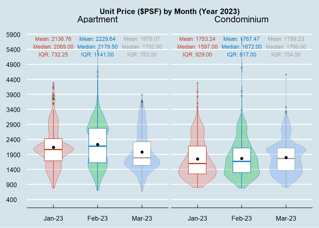
For Year 2024
# Filter and order the data as before
filtered_data <- realis %>%
  filter(PROPERTY_TYPE %in% c("Apartment", "Condominium"),
         MONTH_YEAR %in% c("Jan-24", "Feb-24", "Mar-24")) %>%
  mutate(MONTH_YEAR = factor(MONTH_YEAR, levels = c("Jan-24", "Feb-24", "Mar-24")))

# Calculate summary statistics for annotations
stats_data <- filtered_data %>%
  group_by(MONTH_YEAR, PROPERTY_TYPE) %>%
  summarise(
    Mean = mean(UNIT_PRICE_PSF),
    Median = median(UNIT_PRICE_PSF),
    IQR = IQR(UNIT_PRICE_PSF),
    .groups = 'drop'
  )

# Generate the violin plot with statistical annotations
plot2 <- ggplot(data = filtered_data,
       aes(x = MONTH_YEAR, y = UNIT_PRICE_PSF, color = MONTH_YEAR)) +
  geom_violin(aes(fill = MONTH_YEAR), size = 0.6, alpha = 0.3, linewidth = 0) +
  geom_boxplot(width = 0.4, outlier.colour = "grey20", outlier.size = 1,
               outlier.alpha = 0.3) +
  stat_summary(geom = "point",
               fun.y="mean",
               colour ="black",
               size=2) +
  geom_text(data = stats_data, aes(label = sprintf("Mean: %.2f\nMedian: %.2f\nIQR: %.2f", Mean, Median, IQR),
                                   y = 5500), size = 3, hjust = 0.5) +
  coord_cartesian(ylim = c(400, 6000)) +
  scale_color_manual(values = c("#c73824", "#0477bf", "#9E9E9E", "#0CDBBC")) +
  theme_economist() +
  labs(title = "Unit Price ($PSF) by Month (Year 2024)") +
  scale_y_continuous(breaks = seq(400, 6000, by = 500)) +
  theme(axis.title.x = element_blank(),
        axis.title.y = element_blank(),
        plot.title = element_text(size = 12, hjust = 0.5),
        axis.text = element_text(size = 10),
        legend.position = "none") +
  facet_wrap(~PROPERTY_TYPE)

# Display the plot
print(plot2)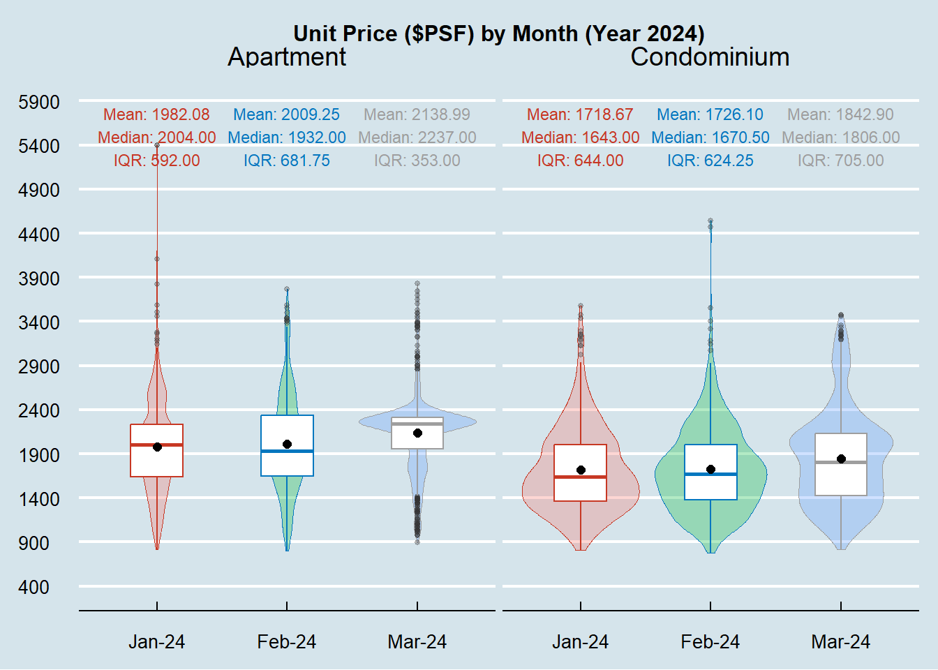
5th iteration (Highlighting Outliers)
# Filter and order the data as before
filtered_data <- realis %>%
  filter(PROPERTY_TYPE %in% c("Apartment", "Condominium"),
         MONTH_YEAR %in% c("Jan-23", "Feb-23", "Mar-23")) %>%
  mutate(MONTH_YEAR = factor(MONTH_YEAR, levels = c("Jan-23", "Feb-23", "Mar-23")))

# Calculate summary statistics for annotations
stats_data <- filtered_data %>%
  group_by(MONTH_YEAR, PROPERTY_TYPE) %>%
  summarise(
    Mean = mean(UNIT_PRICE_PSF),
    Median = median(UNIT_PRICE_PSF),
    IQR = IQR(UNIT_PRICE_PSF),
    .groups = 'drop'
  )

# Generate the violin plot with statistical annotations
plot1 <- ggplot(data = filtered_data,
       aes(x = MONTH_YEAR, y = UNIT_PRICE_PSF, color = MONTH_YEAR)) +
  geom_violin(aes(fill = MONTH_YEAR), size = 0.6, alpha = 0.3, linewidth = 0) +
  geom_boxplot(width = 0.4, outlier.colour = "darkred", outlier.size = 1, outlier.shape = 8,
               outlier.alpha = 0.8) +
  stat_summary(geom = "point",
               fun.y="mean",
               colour ="black",
               size=2) +
  geom_text(data = stats_data, aes(label = sprintf("Mean: %.2f\nMedian: %.2f\nIQR: %.2f", Mean, Median, IQR),
                                   y = 5500), size = 3, hjust = 0.5) +
  coord_cartesian(ylim = c(400, 6000)) +
  scale_color_manual(values = c("#c73824", "#0477bf", "#9E9E9E", "#0CDBBC")) +
  theme_economist() +
  labs(title = "Unit Price ($PSF) by Month (Year 2023)") +
  scale_y_continuous(breaks = seq(400, 6000, by = 500)) +
  theme(axis.title.x = element_blank(),
        axis.title.y = element_blank(),
        plot.title = element_text(size = 12, hjust = 0.5),
        axis.text = element_text(size = 10),
        legend.position = "none") +
  facet_wrap(~PROPERTY_TYPE)

# Display the plot
print(plot1)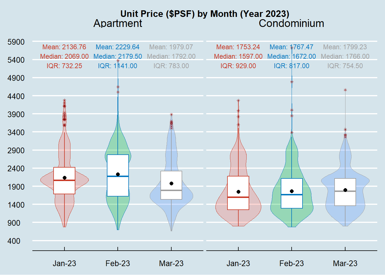
4 Improved Visualisation
Show the code
# Filter and order the data as before
filtered_data <- realis %>%
  filter(PROPERTY_TYPE %in% c("Apartment", "Condominium"),
         MONTH_YEAR %in% c("Jan-24", "Feb-24", "Mar-24")) %>%
  mutate(MONTH_YEAR = factor(MONTH_YEAR, levels = c("Jan-24", "Feb-24", "Mar-24")))

# Calculate summary statistics for annotations
stats_data <- filtered_data %>%
  group_by(MONTH_YEAR, PROPERTY_TYPE) %>%
  summarise(
    Mean = mean(UNIT_PRICE_PSF),
    Median = median(UNIT_PRICE_PSF),
    IQR = IQR(UNIT_PRICE_PSF),
    .groups = 'drop'
  )

# Generate the violin plot with statistical annotations
plot1 <- ggplot(data = filtered_data,
       aes(x = MONTH_YEAR, y = UNIT_PRICE_PSF, color = MONTH_YEAR)) +
  geom_violin(aes(fill = MONTH_YEAR), size = 0.6, alpha = 0.3, linewidth = 0) +
  geom_boxplot(width = 0.4, outlier.colour = "darkred", outlier.size = 1, outlier.shape = 8,
               outlier.alpha = 0.8) +
  stat_summary(geom = "point",
               fun.y="mean",
               colour ="black",
               size=2) +
  geom_text(data = stats_data, aes(label = sprintf("Mean: %.2f\nMedian: %.2f\nIQR: %.2f", Mean, Median, IQR),
                                   y = 5500), size = 3, hjust = 0.5) +
  coord_cartesian(ylim = c(400, 6000)) +
  scale_color_manual(values = c("#c73824", "#0477bf", "#9E9E9E", "#0CDBBC")) +
  theme_economist() +
  labs(title = "Unit Price ($PSF) by Month (Year 2024)") +
  scale_y_continuous(breaks = seq(400, 6000, by = 500)) +
  theme(axis.title.x = element_blank(),
        axis.title.y = element_blank(),
        plot.title = element_text(size = 12, hjust = 0.5),
        axis.text = element_text(size = 10),
        legend.position = "none") +
  facet_wrap(~PROPERTY_TYPE)

# Display the plot
print(plot1)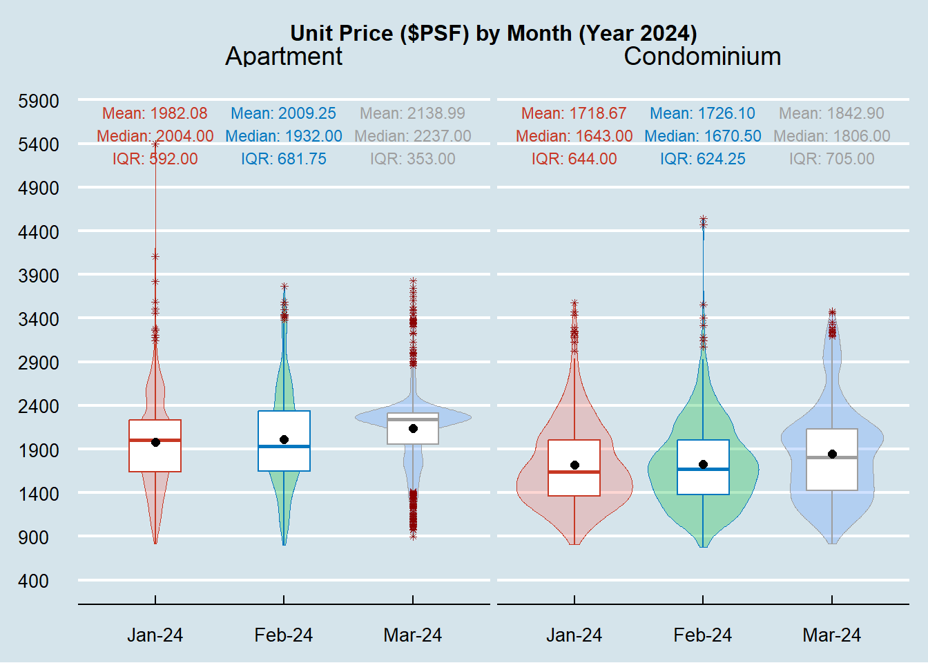
Show the code
# Filter and order the data as before
filtered_data <- realis %>%
  filter(PROPERTY_TYPE %in% c("Apartment", "Condominium"),
         MONTH_YEAR %in% c("Jan-23", "Feb-23", "Mar-23")) %>%
  mutate(MONTH_YEAR = factor(MONTH_YEAR, levels = c("Jan-23", "Feb-23", "Mar-23")))

# Calculate summary statistics for annotations
stats_data <- filtered_data %>%
  group_by(MONTH_YEAR, PROPERTY_TYPE) %>%
  summarise(
    Mean = mean(UNIT_PRICE_PSF),
    Median = median(UNIT_PRICE_PSF),
    IQR = IQR(UNIT_PRICE_PSF),
    .groups = 'drop'
  )

# Generate the violin plot with statistical annotations
plot1 <- ggplot(data = filtered_data,
       aes(x = MONTH_YEAR, y = UNIT_PRICE_PSF, color = MONTH_YEAR)) +
  geom_violin(aes(fill = MONTH_YEAR), size = 0.6, alpha = 0.3, linewidth = 0) +
  geom_boxplot(width = 0.4, outlier.colour = "darkred", outlier.size = 1, outlier.shape = 8,
               outlier.alpha = 0.8) +
  stat_summary(geom = "point",
               fun.y="mean",
               colour ="black",
               size=2) +
  geom_text(data = stats_data, aes(label = sprintf("Mean: %.2f\nMedian: %.2f\nIQR: %.2f", Mean, Median, IQR),
                                   y = 5500), size = 3, hjust = 0.5) +
  coord_cartesian(ylim = c(400, 6000)) +
  scale_color_manual(values = c("#c73824", "#0477bf", "#9E9E9E", "#0CDBBC")) +
  theme_economist() +
  labs(title = "Unit Price ($PSF) by Month (Year 2023)") +
  scale_y_continuous(breaks = seq(400, 6000, by = 500)) +
  theme(axis.title.x = element_blank(),
        axis.title.y = element_blank(),
        plot.title = element_text(size = 12, hjust = 0.5),
        axis.text = element_text(size = 10),
        legend.position = "none") +
  facet_wrap(~PROPERTY_TYPE)

# Display the plot
print(plot1)
5 Key Takeaways
Overall, the selected peer’s work was done up relatively well.
The processes for the data visualisation makeover in this take-home exercise illustrates the utmost importance of attention to detail when making a plot. Here are some pointers which I found were useful:
To check the data
- It goes without saying that data is the core element of any chart or graph. If the data is unreliable, the graph will also be unreliable. Therefore, it’s crucial to ensure your data is accurate. Begin by creating straightforward graphs to identify any outliers or unusual spikes. Always double-check anything that looks off. You may find a surprising number of data entry errors in the spreadsheets you receive.
Choosing of colours
- Effective use of color can significantly enhance and clarify a presentation, while poor use of color can lead to confusion and obscurity. Although color adds an aesthetic quality, its primary role in displaying information is functional. The key is to consider what information needs to be conveyed and to determine if and how color can improve the communication of that information.
Highlighting what’s important
- To effectively communicate a message, it’s essential to direct your audience’s attention to the data under analysis. Start with a title that captures the essence of your insight. Then, emphasize your data visually while maintaining other data in a subdued manner in the background, providing context and enabling comparisons.
6 References
URA releases flash estimate of 1st Quarter 2024 private residential property price index
Unsold private housing stock on the rise ahead of ramp-up in new launches in 2024
HDB resale prices rise 1.7%; private home prices up 1.5% in first quarter: Flash estimates
Dos and don’ts of data visualisation — European Environment Agency