In-class Exercise 6b

6.0 VAST Challenge 2024 - MC3

6.1 Loading the necessary R packages

pacman::p_load(jsonlite, tidygraph, ggraph,
               visNetwork, graphlayouts, ggforce,
               skimr, tidytext, tidyverse)

6.2 Data import

In the code chunk below, fromJSON() of jsonlite package is used to import MC3.json into the R environment

mc3_data <- fromJSON("data/MC3.json")

In the code chunk below the class() function is used to confirm that the data is imported as a list

class(mc3_data)

[1] "list"

The output is called mc3_data. It is a large list R object.

6.3 Extracing edges

The code chunk below will be used to extract the links data.frame of mc3_data and saves it as a tibble data.frame called mc3_edges.

mc3_edges <-
  as_tibble(mc3_data$links) %>%
  distinct() %>% #to avoid duplicate records; source,target,type if they are the same will be treated as duplicates and kept as one
  mutate(source = as.character(source),
         target = as.character(target),
         type = as.character(type)) %>%
  group_by(source, target, type) %>%
    summarise(weights = n()) %>% #weight - representation the number of linkages
  filter(source!=target) %>%
  ungroup()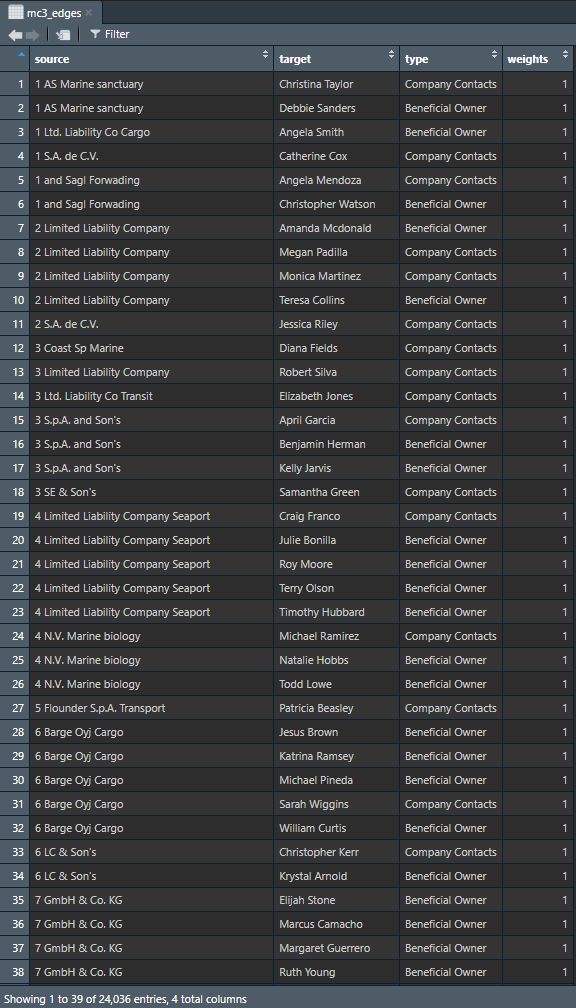

MC3 Edges tibble data.frame

In the code chunk above

• distinct() is used to ensure that there will be no duplicated records.
• mutate() and as.character() are used to convert the field data type from list to character.
• group_by() and summarise() are used to count the number of unique links
• the filter(source!=target) is to ensure that no records are with similar source and target.

6.4 Extracing nodes

mc3_nodes <- as.tibble(mc3_data$nodes) %>% #extracting from the nodes data.frame
  mutate(country = as.character(country),
         id = as.character(id),
         product_services = as.character(product_services),
         revenue_omu = as.numeric(as.character(revenue_omu)), #as.numeric() since revenue should be processed as number to be able to do statistical analysis such as average
         type = as.character(type)) %>%
  select(id, country, type, revenue_omu, product_services)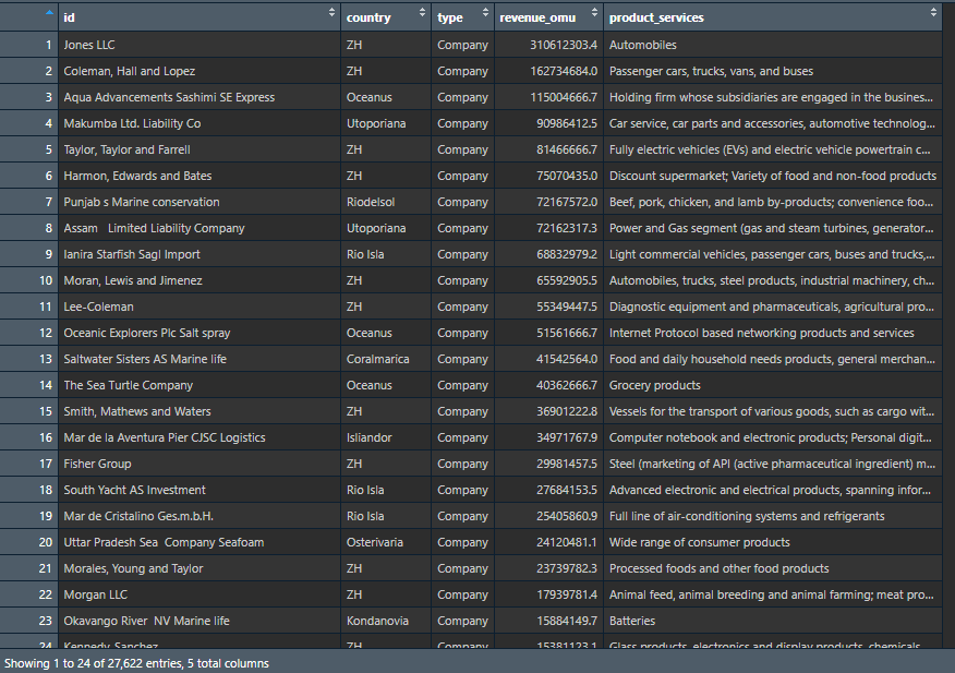

MC3 Nodes tibble data.frame

In the code chunk above

• to convert revenue_omu from list data type to numeric data type, we would have to convert the values into character first by using as.character() followed by as.numeric() to convert the data into numeric data type.
• select() is used to re-organise the order of the fields.

6.5 Initial data exploration

Exploring the edges data frame

In the code chunk below, [skim()])(https://docs.ropensci.org/skimr/reference/skim.html) of skimr package is used to display the summary statistics of mc3_edges tibble data.frame.

skim(mc3_edges)

Data summary

Name	mc3_edges
Number of rows	24036
Number of columns	4
_______________________
Column type frequency:
character	3
numeric	1
________________________
Group variables	None

Variable type: character

skim_variable	n_missing	complete_rate	min	max	empty	n_unique	whitespace
source	0	1	6	700	0	12856	0
target	0	1	6	28	0	21265	0
type	0	1	16	16	0	2	0

Variable type: numeric

skim_variable	n_missing	complete_rate	mean	sd	p0	p25	p50	p75	p100	hist
weights	0	1	1	0	1	1	1	1	1	▁▁▇▁▁

The code function reveals that there is no missing value in the fields.

In the code chunk below, datatable() of DT package is used to display mc3_edges tibble data.frame as an interactive table on the html document.

DT::datatable(mc3_edges)

ggplot(data = mc3_edges,
       aes(x = type)) +
  geom_bar() +
  geom_text(aes(label = type), stat = "count", vjust = 5.5, colour = "white")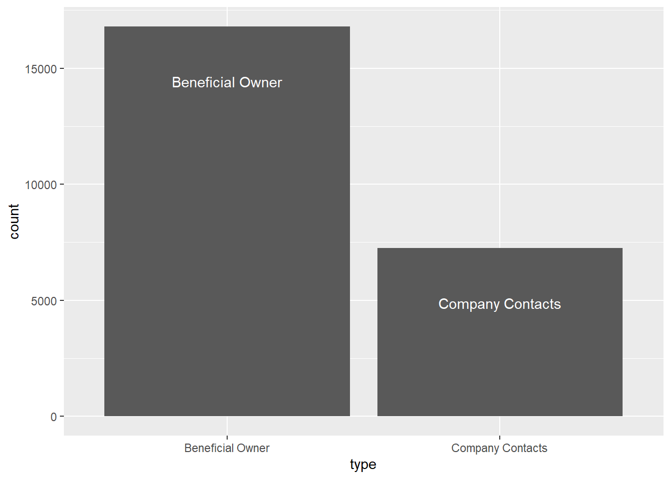

6.6 Building network model with tidygraph

6.6.1 Preparing the network graph

In the code chunk below,

• since some data were trimmed away, the nodes and edges might not sync together
• from the code below, we pull out the name/ create a new node from the edges to represent source and target
• purpose is to update the nodes based on the new edges data in the R environment
• followed by combining id1 & id2 and using left_join() to append them back to mc3_nodes

id1 <- mc3_edges %>%
  select(source) %>%
  rename(id = source)
id2 <- mc3_edges %>%
  select(target) %>%
  rename(id = target)
mc3_nodes1 <- rbind(id1, id2) %>%
  distinct() %>%
  left_join(mc3_nodes,
            unmatched = 'drop')

6.6.2 To construct the graph model

mc3_graph <- tbl_graph(nodes = mc3_nodes1,
                       edges = mc3_edges,
                       directed = FALSE) %>%
  mutate(betweenness_centrality =  # field name
centrality_betweenness(),  # function - from tidygraph; nested function within the graph
          closeness_centrality =
centrality_closeness())

Building the graph to visualise

betweenness_centrality >= 100000

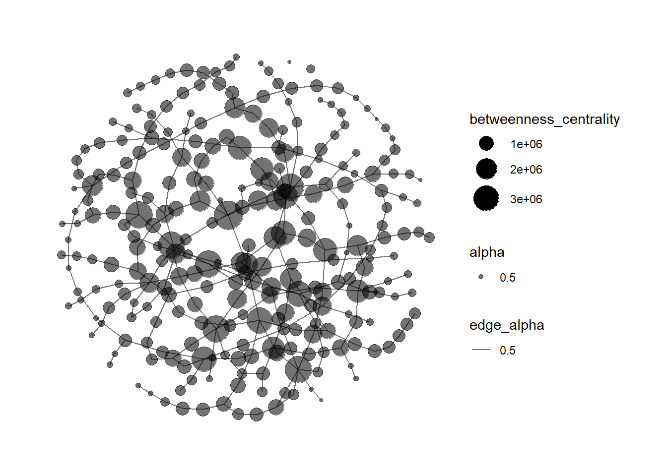
mc3_graph %>%
    filter(betweenness_centrality >= 100000) %>% #`filter()` function used pull out nodes with betweenness centrality greater than input value.
ggraph(layout = "fr") +
  geom_edge_link(aes(alpha=0.5)) +
  geom_node_point(aes(
    size = betweenness_centrality,
    colors = "lightblue",
    alpha = 0.5)) +
  scale_size_continuous(range = c(1,10)) +
  theme_graph()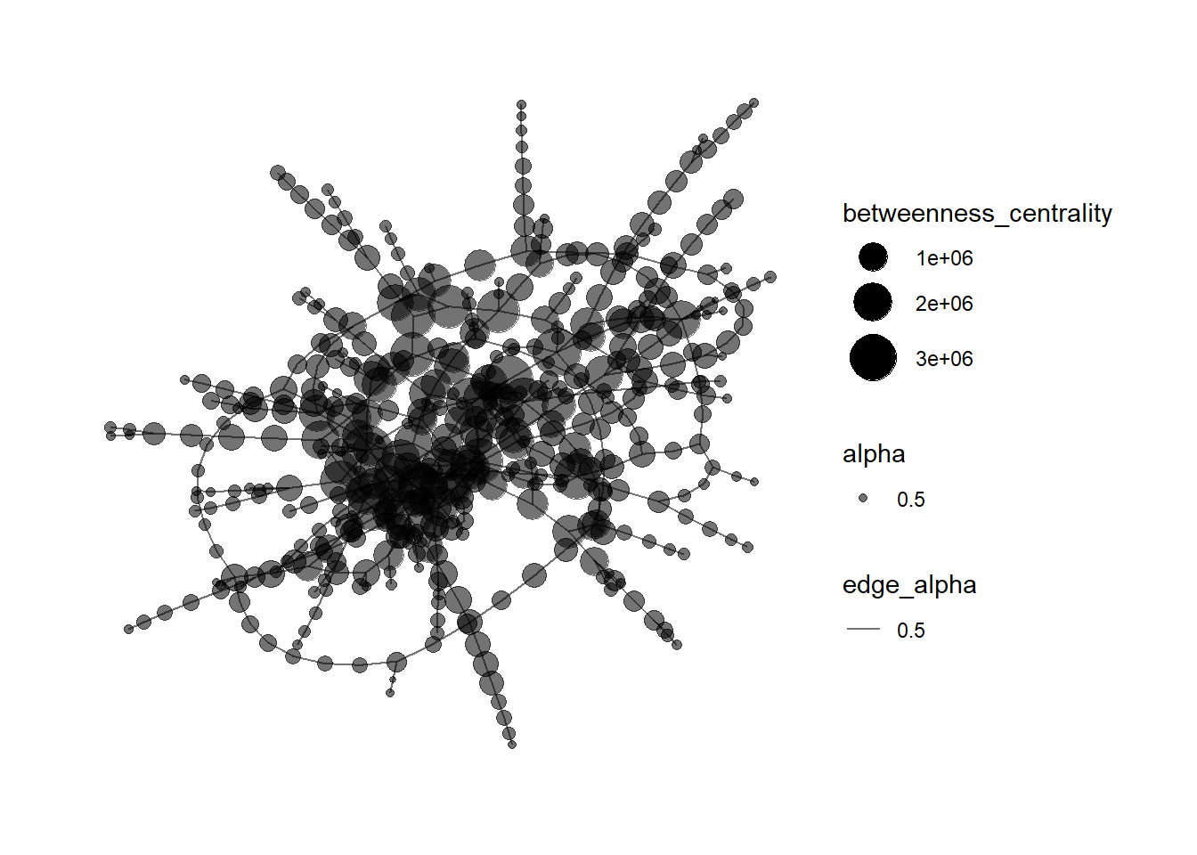

betweenness_centrality >= 300000

increased betweenness_centrality from 100000 to 300000;

mc3_graph %>%
    filter(betweenness_centrality >= 300000) %>% #`filter()` function is used to pull out nodes with betweenness centrality greater than 300000 to avoid the graph being too cluttered.
ggraph(layout = "fr") +
  geom_edge_link(aes(alpha=0.5)) +
  geom_node_point(aes(
    size = betweenness_centrality,
    colors = "lightblue",
    alpha = 0.5)) +
  scale_size_continuous(range = c(1,10)) +
  theme_graph()