Take-home Exercise 3: Network Data Visualisation and Analysis

Author

Ho Zi Jun

Published

June 9, 2024

Modified

June 13, 2024

1 VAST Challenge: Mini-Challenge 3

1.1 Background and Overview

Oceanus has a dynamic business landscape with frequent startups, mergers, acquisitions and investments. FishEye International, a non-profit organization that focuses on illegal fishing monitors commercial fishing operators to prevent illegal fishing in the region’s sensitive marine ecosystem. Analysts use a hybrid automated/manual process to transform company records into CatchNet: the Oceanus Knowledge Graph.

Last year, SouthSeafood Express Corp was caught fishing illegally, disrupting the commercial fishing sector. FishEye aims to analyse the temporal patterns and impacts of this incident on the fishing market. The competitive nature of the market might lead some businesses attempting to seize SouthSeafood’s market share, while others may recognize the consequences of illegal fishing.

2 Project Objectives

The project will focus on 2 out of the 4 tasks (Questions 3 and 4) from VAST Challenge 2024: Mini-Challenge 3

This project aims to develop visualisation tools that work with CatchNet to identify the people who hold influence over business networks and hold those who own nefarious companies accountable. That is especially difficult with varied and changing shareholder and ownership relationships. The tasks are:

Develop a visual approach to examine inferences. Infer how the influence of a company changes through time. Can we infer ownership or influence that a network may have?

Identify the network associated with SouthSeafood Express Corp and visualize how this network and competing businesses change as a result of their illegal fishing behavior. Which companies benefited from SouthSeafood Express Corp legal troubles? Are there other suspicious transactions that may be related to illegal fishing? Providing visual evidence for the conclusions.

Note: the VAST challenge is focused on visual analytics and graphical figures should be included with your response to each question. Please include a reasonable number of figures for each question (no more than about 6) and keep written responses as brief as possible (around 250 words per question). Participants are encouraged to new visual representations rather than relying on traditional or existing approaches.

3 Hypothesis and Methodology

For these questions, we would have to investigate the changes through time in multiple areas mainly:

Individual’s ownership and influence on a network for the first portion
Following which, how the networks and companies changes as a result of the SouthSeafood Express Corp incident.

To achieve this we will attempt to create visualisations of network graphs and carrying out faceting to allow us to observe for patterns and trends and make our inferences.

%%{
  init: {
    "theme": "base",
    "themeVariables": {
      "primaryColor": "#d8e8e6",
      "primaryTextColor": "#325985",
      "primaryBorderColor": "#325985",
      "lineColor": "#325985",
      "secondaryColor": "#cedded",
      "tertiaryColor": "#fff" 
      }
  }
}%%

flowchart LR
    A[Person / CEO] -->|Ownership\n OR \nInfluence| B(Organisation)
    B ---> C{Company}
    B ---> D{FishingCompany}
    B ---> E{LogisticsCompany}
    B ---> F{NewsCompany}
    B ---> G{FinancialCompany}
    B ---> H{NGO}

%%{
  init: {
    "theme": "base",
    "themeVariables": {
      "primaryColor": "#d8e8e6",
      "primaryTextColor": "#325985",
      "primaryBorderColor": "#325985",
      "lineColor": "#325985",
      "secondaryColor": "#cedded",
      "tertiaryColor": "#fff" 
      }
  }
}%%
   
flowchart LR
  A[Companies] --> |BENEFITED| B(SouthSeafood Express Corp)
  C{Suspicious\nTranscations}
  C --> A
  C --> E[Illegal Fishing]

4 Getting Started

4.1 Installing and launching R packages

In the code chunk below, p_load() of pacman package is used to check if the following packages have been installed and also will load them into the working R environment.

The code chunk:

Code

pacman::p_load(jsonlite, tidygraph, ggraph, visNetwork, knitr,
               graphlayouts, ggforce, tidyverse, tidytext, RColorBrewer,
               skimr, DT, lubridate, plotly, clock, igraph)

4.2 The Data

In the code chunk below, fromJSON() of jsonlite package is used to import MC3.json file into the R environment.

Code

mc3_data <- fromJSON("data/MC3/mc3.json")

Initially, when trying to load the mc3.json data we faced an error message regarding a NaN issue.

Error message Hence we converted solely the NaN fields to “NaN” to curb this issue and the mc3.json file is imported successfully.

Code

class(mc3_data)

[1] "list"

The output is called mc3_data. It is a large list R object. There are two data frames. One contains the nodes data and the other contains the edges (also know as link) data.

Code

mc3_edges <- as_tibble(mc3_data$links) %>% 
  unnest(source) %>% 
  distinct() %>% 
  mutate(source = as.character(source),
         target = as.character(target),
         type = as.character(type),
         startdate = as_datetime(start_date)) %>% 
  group_by(source, target, type, startdate) %>% 
  summarise(weights = n()) %>% 
  filter(source != target) %>%
  ungroup()

head(mc3_edges)

# A tibble: 6 × 5
  source                 target                type  startdate           weights
  <chr>                  <chr>                 <chr> <dttm>                <int>
1 4. SeaCargo Ges.m.b.H. Dry CreekRybachit Ma… Even… 2034-12-31 00:00:00       1
2 4. SeaCargo Ges.m.b.H. KambalaSea Freight I… Even… 2033-04-12 00:00:00       1
3 9. RiverLine CJSC      SumacAmerica Transpo… Even… 2028-12-02 00:00:00       1
4 Aaron Acosta           Manning-Pratt         Even… 2008-09-14 00:00:00       1
5 Aaron Acosta           Manning-Pratt         Even… 2008-07-30 00:00:00       1
6 Aaron Allen            Hicks-Calderon        Even… 2025-03-06 00:00:00       1

Code

ggplot(data = mc3_edges, aes(x = type)) +
  geom_bar()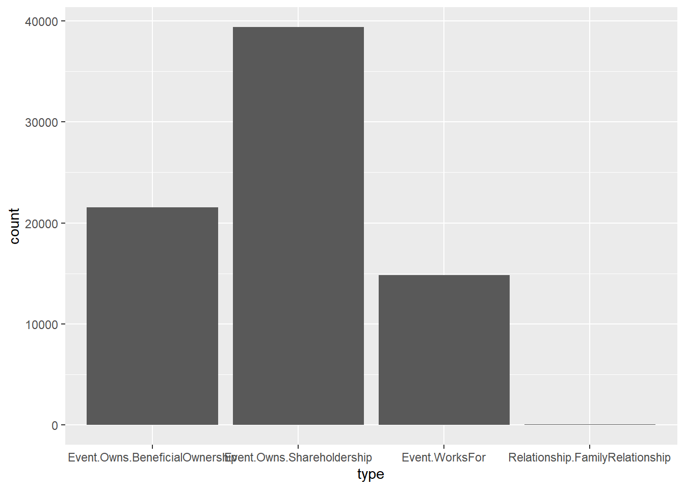

From the type field, we can see that there are four types of edges with FamilyRelationship edges only having type attributes as stated in the VAST 2024 - MC3 Data Description.

Code

# extract all nodes from graph
mc3_nodes <- as_tibble(mc3_data$nodes) %>% 
  mutate(country = as.character(country),
         id = as.character(id),
         revenue = as.numeric(as.character(revenue)),
         type = as.character(type)) %>%
  select(id, country, type, revenue)

# extract all nodes from edges
id1 <- mc3_edges %>%
  select(source, type) %>%
  rename(id = source) %>% 
  mutate(country = NA, revenue = NA) %>% 
  select(id, country, type, revenue)

id2 <- mc3_edges %>%
  select(target, type) %>%
  rename(id = target) %>% 
  mutate(country = NA, revenue = NA) %>% 
  select(id, country, type, revenue)

additional_nodes <- rbind(id1, id2) %>% 
  distinct %>% 
  filter(!id %in% mc3_nodes[["id"]])

# combine all nodes
mc3_nodes_updated <- rbind(mc3_nodes, additional_nodes) %>%
  distinct()

head(mc3_nodes_updated)

# A tibble: 6 × 4
  id                          country     type                        revenue
  <chr>                       <chr>       <chr>                         <dbl>
1 Abbott, Mcbride and Edwards Uziland     Entity.Organization.Company   5995.
2 Abbott-Gomez                Mawalara    Entity.Organization.Company  71767.
3 Abbott-Harrison             Uzifrica    Entity.Organization.Company      0 
4 Abbott-Ibarra               Islavaragon Entity.Organization.Company      0 
5 Abbott-Sullivan             Oceanus     Entity.Organization.Company   4747.
6 Acevedo and Sons            Imazam      Entity.Organization.Company  46567.

Code

ggplot(data = mc3_nodes_updated, aes(x = type)) +
  geom_bar()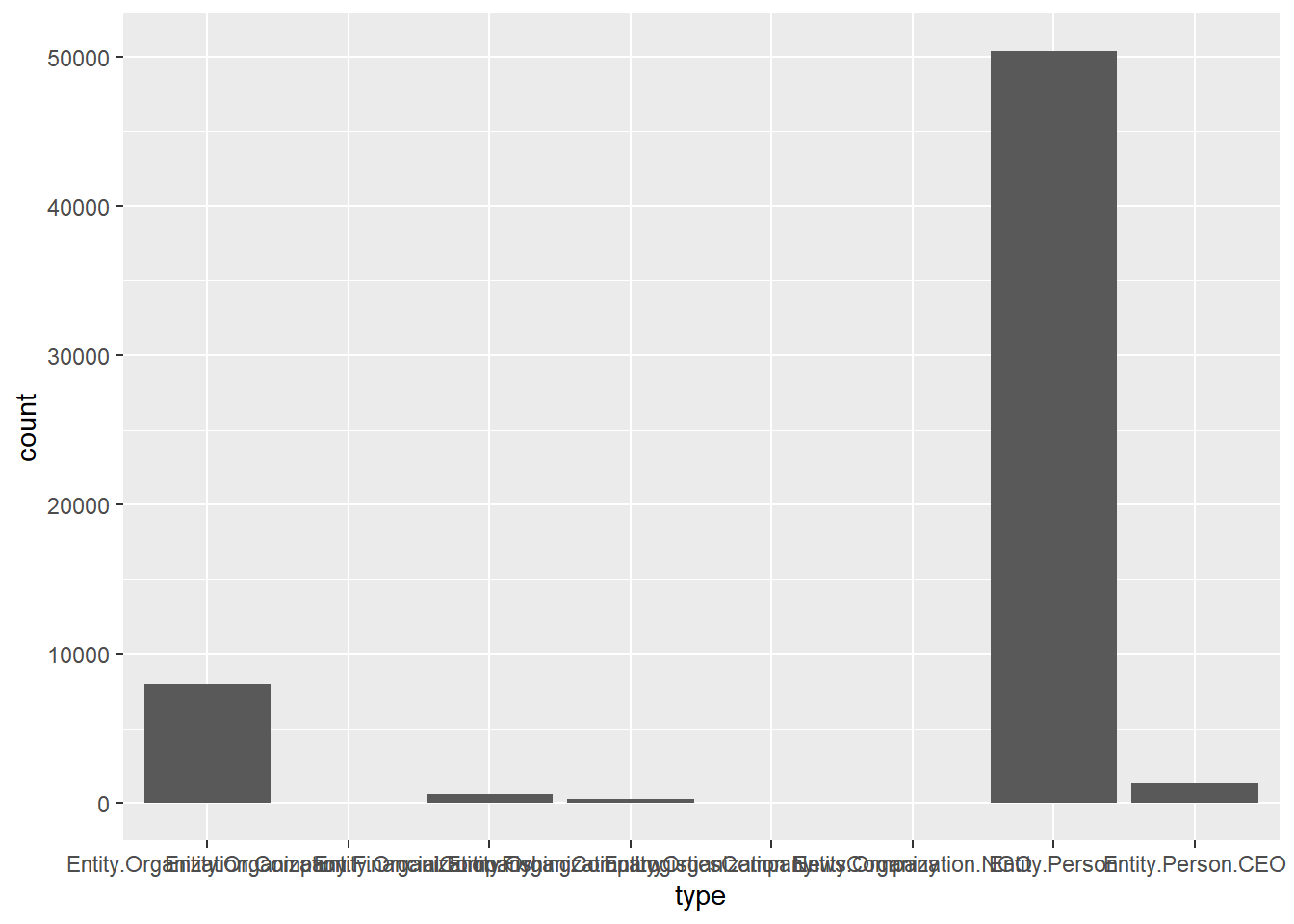

Code

mc3_nodes_updated[duplicated(mc3_nodes_updated$id),] %>% 
  arrange(id)

# A tibble: 0 × 4
# ℹ 4 variables: id <chr>, country <chr>, type <chr>, revenue <dbl>

No Duplicates

Code

mc3_nodes_master <- mc3_nodes_updated %>% 
  group_by(id) %>% 
  arrange(id, type, country) %>% 
  summarise(countries = paste0(unique(country), collapse = ", "),
            num_countries = n_distinct(country),
            types = paste0(unique(type), collapse = ", "),
            num_types = n_distinct(type),
            revenue = sum(revenue))

Code

# form graph
mc3_graph <- tbl_graph(nodes = mc3_nodes_master,
                       edges = mc3_edges,
                       directed = FALSE) %>% 
  mutate(betweenness_centrality = centrality_betweenness())

# extract node with highest betweenness centrality
top1_betw <- mc3_graph %>% 
  activate(nodes) %>% 
  as_tibble() %>% 
  top_n(1, betweenness_centrality) %>% 
    select(id, countries, types)

# extract lvl 1 edges
top1_betw_edges_lvl1 <- mc3_edges %>% 
  filter(source %in% top1_betw[["id"]] | target %in% top1_betw[["id"]])

# extract nodes from lvl 1 edges
id1 <- top1_betw_edges_lvl1 %>%
  select(source) %>%
  rename(id = source) %>% 
  left_join(mc3_nodes_master, by = "id") %>% 
  select(id, countries, types)

id2 <- top1_betw_edges_lvl1 %>%
  select(target) %>%
  rename(id = target) %>% 
  left_join(mc3_nodes_master, by = "id") %>% 
  select(id, countries, types)

additional_nodes_lvl1 <- rbind(id1, id2) %>% 
  distinct %>% 
  filter(!id %in% top1_betw[["id"]])

# extract lvl 2 edges
top1_betw_edges_lvl2 <- mc3_edges %>% 
  filter(source %in% additional_nodes_lvl1[["id"]] | target %in% additional_nodes_lvl1[["id"]])

# extract nodes from lvl 1 edges
id1 <- top1_betw_edges_lvl2 %>%
  select(source) %>%
  rename(id = source) %>% 
  left_join(mc3_nodes_master, by = "id") %>% 
  select(id, countries, types)

id2 <- top1_betw_edges_lvl2 %>%
  select(target) %>%
  rename(id = target) %>% 
  left_join(mc3_nodes_master, by = "id") %>% 
  select(id, countries, types)

additional_nodes_lvl2 <- rbind(id1, id2) %>% 
  distinct %>% 
  filter(!id %in% top1_betw[["id"]] & !id %in% additional_nodes_lvl1[["id"]])

# combine all nodes
top1_betw_nodes <- rbind(top1_betw, additional_nodes_lvl1, additional_nodes_lvl2) %>%
  distinct()

# combine all edges
top1_betw_edges <- rbind(top1_betw_edges_lvl1, top1_betw_edges_lvl2) %>% 
  distinct()

# colur palatte for betweenness centrality colours
sw_colors <- colorRampPalette(brewer.pal(3, "RdBu"))(3)

# customise edges for plotting
top1_betw_edges <- top1_betw_edges %>% 
  rename(from = source,
         to = target) %>% 
  mutate(title = paste0("Type: ", type), # tooltip when hover over
         color = "#0085AF") # color of edge

# customise nodes for plotting
top1_betw_nodes <- top1_betw_nodes %>% 
  rename(group = types) %>% 
  mutate(id.type = ifelse(id == top1_betw[["id"]], sw_colors[1], sw_colors[2])) %>%
  mutate(title = paste0(id, "<br>Group: ", group), # tooltip when hover over
         size = 30, # set size of nodes
         color.border = "#013848", # border colour of nodes
         color.background = id.type, # background colour of nodes
         color.highlight.background = "#FF8000" # background colour of nodes when highlighted
         )

# plot graph
visNetwork(top1_betw_nodes, top1_betw_edges,
           height = "500px", width = "100%",
           main = paste0("Network Graph of ", top1_betw[["id"]])) %>%
  visIgraphLayout() %>%
  visGroups(groupname = "Entity.Organization.Company", shape = "triangle") %>%
  visGroups(groupname = "Entity.Organization.Company, Entity.Organization.FishingCompany", shape = "triangle") %>%
  visGroups(groupname = "Entity.Organization.Company, Entity.Organization.FishingCompany, Entity.Organization.LogisticsCompany", shape = "triangle") %>%
  visGroups(groupname = "Entity.Organization.Company, Entity.Organization.FishingCompany, Entity.Organization.LogisticsCompany, Entity.Organization.FinancialCompany", shape = "triangle") %>%
  visGroups(groupname = "Entity.Organization.Company, Entity.Organization.FishingCompany, Entity.Organization.LogisticsCompany, Entity.Organization.FinancialCompany, Entity.Organization.NewsCompany", shape = "triangle") %>%
  visGroups(groupname = "Entity.Organization.Company, Entity.Organization.FishingCompany, Entity.Organization.LogisticsCompany, Entity.Organization.FinancialCompany, Entity.Organization.NewsCompany, Entity.Organization.NGO", shape = "triangle") %>%
  visOptions(selectedBy = "group",
             highlightNearest = list(enabled = T, degree = 1, hover = T),
             nodesIdSelection = TRUE) %>% 
  visLayout(randomSeed = 123)

Perform analysis on largest components in the network:

Code

# form graph
mc3_graph <- tbl_graph(nodes = mc3_nodes_master,
                       edges = mc3_edges,
                       directed = FALSE)

# find components in graph
set.seed(123)
clusters <- components(mc3_graph)

# update graph with component membership
mc3_nodes_master <- mc3_nodes_master %>% 
  mutate(component_membership = clusters$membership)

# extract info relating to components
component_df <- clusters$csize %>% 
  as_tibble() %>% 
  rownames_to_column() %>% 
  rename(component_membership = rowname,
         component_size = value)

# find components that are top 3 in size    
top_3_components <- component_df %>% 
  top_n(3, component_size) %>% 
  arrange(desc(component_size))

datatable(top_3_components)

Next, we will visualise the network charts of the three largest clusters separately using interactive charts below.

Code

visualise_cluster <- function(x){
  
# extract nodes in component
component_nodes <- mc3_nodes_master %>%
  filter(component_membership == x)

# extract edges in component
component_edges <- mc3_edges %>% 
  filter(source %in% component_nodes[["id"]] | target %in% component_nodes[["id"]])

# compute centrality measures
component_graph <- tbl_graph(nodes = component_nodes,
                             edges = component_edges,
                             directed = FALSE) %>% 
  mutate(closeness_centrality = centrality_closeness(),
         betweenness_centrality = centrality_betweenness(),
         eigen_cetrality = centrality_eigen())

# compute the top 90th percentile centrality
component_nodes_updated <- component_graph %>% 
  activate(nodes) %>% 
  as_tibble()

cent_per_90 <- quantile(component_nodes_updated$betweenness_centrality,
                               probs = 0.90)

component_nodes_updated <- component_nodes_updated %>% 
  mutate(is_top_cent_90 = ifelse(betweenness_centrality >= cent_per_90, "yes", "no"))

# colur palatte for betweenness centrality colours
sw_colors <- colorRampPalette(brewer.pal(3, "RdBu"))(3)

# customise edges for plotting
component_edges <- component_edges %>% 
  rename(from = source,
         to = target) %>% 
  mutate(title = paste0("Type: ", type), # tooltip when hover over
         color = "#0085AF") # color of edge

# customise nodes for plotting
component_nodes_updated <- component_nodes_updated %>% 
  rename(group = types) %>% 
  mutate(is_top_cent_90.type = ifelse(is_top_cent_90 == "yes", sw_colors[1], sw_colors[2])) %>% 
  mutate(title = paste0(id, "<br>Group: ", group), # tooltip when hover over
         size = 40, # set size of nodes
         color.border = "#013848", # border colour of nodes
         color.background = is_top_cent_90.type, # background colour of nodes
         color.highlight.background = "#FF8000" # background colour of nodes when highlighted
         )

# plot graph
visNetwork(component_nodes_updated, component_edges,
           height = "500px", width = "100%",
           main = paste0("Entities in Component ", x)) %>%
  visIgraphLayout() %>%
  visGroups(groupname = "Entity.Organization.Company", shape = "triangle") %>%
  visGroups(groupname = "Entity.Organization.Company, Entity.Organization.FishingCompany", shape = "triangle") %>%
  visGroups(groupname = "Entity.Organization.Company, Entity.Organization.FishingCompany, Entity.Organization.LogisticsCompany", shape = "triangle") %>%
  visGroups(groupname = "Entity.Organization.Company, Entity.Organization.FishingCompany, Entity.Organization.LogisticsCompany, Entity.Organization.FinancialCompany", shape = "triangle") %>%
  visGroups(groupname = "Entity.Organization.Company, Entity.Organization.FishingCompany, Entity.Organization.LogisticsCompany, Entity.Organization.FinancialCompany, Entity.Organization.NewsCompany", shape = "triangle") %>%
  visGroups(groupname = "Entity.Organization.Company, Entity.Organization.FishingCompany, Entity.Organization.LogisticsCompany, Entity.Organization.FinancialCompany, Entity.Organization.NewsCompany, Entity.Organization.NGO", shape = "triangle") %>%
  visGroups(groupname = "Entity.Organization.Company, Entity.Organization.FishingCompany, Entity.Organization.LogisticsCompany, Entity.Organization.FinancialCompany, Entity.Organization.NewsCompany, Entity.Organization.NGO, Entity.Person", shape = "triangle") %>%
  visGroups(groupname = "Entity.Organization.Company, Entity.Organization.FishingCompany, Entity.Organization.LogisticsCompany, Entity.Organization.FinancialCompany, Entity.Organization.NewsCompany, Entity.Organization.NGO, Entity.Person, Entity.Person.CEO", shape = "triangle") %>%
  visOptions(selectedBy = "group",
             highlightNearest = list(enabled = T, degree = 1, hover = T),
             nodesIdSelection = TRUE) %>% 
  visLayout(randomSeed = 123)

}

visualise_cluster(1)

Code

visualise_cluster(504)

5 Data Wrangling

In order to improve the data quality and make it more consumable and useful for analytics, we will proceed with data wrangling to transform and structure the raw data form into specific desired formats

In this section, we will extract and wrangle the edges object. The edges form the relationship or link between different nodes.

5.1.1 Extracting the edges data

The code chunk below will be used to extract the links data.frame of mc3_data and saves it as a tibble data.frame called mc3_edges_raw.

Code

mc3_edges_raw <- as_tibble(mc3_data$links) %>%
  distinct() #use to avoid duplicate records; if they are the same will be treated as duplicates and kept as one

glimpse() of dplyr will be used to reveal the structure of mc3_edges_raw tibble data.table

Code

glimpse(mc3_edges_raw)

Rows: 75,817
Columns: 11
$ start_date          <chr> "2016-10-29T00:00:00", "2035-06-03T00:00:00", "202…
$ type                <chr> "Event.Owns.Shareholdership", "Event.Owns.Sharehol…
$ `_last_edited_by`   <chr> "Pelagia Alethea Mordoch", "Niklaus Oberon", "Pela…
$ `_last_edited_date` <chr> "2035-01-01T00:00:00", "2035-07-15T00:00:00", "203…
$ `_date_added`       <chr> "2035-01-01T00:00:00", "2035-07-15T00:00:00", "203…
$ `_raw_source`       <chr> "Existing Corporate Structure Data", "Oceanus Corp…
$ `_algorithm`        <chr> "Automatic Import", "Manual Entry", "Automatic Imp…
$ source              <chr> "Avery Inc", "Berger-Hayes", "Bowers Group", "Bowm…
$ target              <chr> "Allen, Nichols and Thompson", "Jensen, Morris and…
$ key                 <int> 0, 0, 0, 0, 0, 0, 0, 0, 0, 0, 0, 0, 0, 0, 0, 0, 0,…
$ end_date            <chr> NA, NA, NA, NA, NA, NA, NA, NA, NA, NA, NA, NA, NA…

Note

The following issues can be identified from the table above:

columns with date data type are not in the correct format
some field names(for e.g _last_edited_by, _date_added) start with “_” and will have to be renamed to avoid unnecessary coding issues in the later part of the tasks.

5.1.2 Correcting the date data type

The code chunk below uses as_datetime() of the lubridate package to convert fields with character date into POSIXt format.

Code

mc3_edges_raw$"start_date" <- as_datetime(mc3_edges_raw$start_date)
mc3_edges_raw$"_last_edited_date" <- as_datetime(mc3_edges_raw$"_last_edited_date")
mc3_edges_raw$"_date_added" <- as_datetime(mc3_edges_raw$"_date_added")
mc3_edges_raw$"end_date" <- as_datetime(mc3_edges_raw$end_date)

5.1.3 Changing field name

In the code chunk below, rename() of dplyr package is used to change the following fields that start with “_”.

Code

mc3_edges_raw <- mc3_edges_raw %>%
  rename("last_edited_by" = "_last_edited_by",
         "last_edited_date" = "_last_edited_date",
         "date_added" = "_date_added",
         "raw_source" = "_raw_source",
         "algorithm" = "_algorithm")

Next, glimpse() function will be used to confirm if the processes above have been performed correctly.

Code

glimpse(mc3_edges_raw)

Rows: 75,817
Columns: 11
$ start_date       <dttm> 2016-10-29, 2035-06-03, 2028-11-20, 2024-09-04, 2034…
$ type             <chr> "Event.Owns.Shareholdership", "Event.Owns.Shareholder…
$ last_edited_by   <chr> "Pelagia Alethea Mordoch", "Niklaus Oberon", "Pelagia…
$ last_edited_date <dttm> 2035-01-01, 2035-07-15, 2035-01-01, 2035-01-01, 2035…
$ date_added       <dttm> 2035-01-01, 2035-07-15, 2035-01-01, 2035-01-01, 2035…
$ raw_source       <chr> "Existing Corporate Structure Data", "Oceanus Corpora…
$ algorithm        <chr> "Automatic Import", "Manual Entry", "Automatic Import…
$ source           <chr> "Avery Inc", "Berger-Hayes", "Bowers Group", "Bowman-…
$ target           <chr> "Allen, Nichols and Thompson", "Jensen, Morris and Do…
$ key              <int> 0, 0, 0, 0, 0, 0, 0, 0, 0, 0, 0, 0, 0, 0, 0, 0, 0, 0,…
$ end_date         <dttm> NA, NA, NA, NA, NA, NA, NA, NA, NA, NA, NA, NA, NA, …

5.1.4 Selecting the columns

We will select the relevant variables for our analysis:

source - to identify the actor of the relationship, corresponds to id in nodes.
target - to identify the receiver of the relationship, corresponds to id in nodes.
type - to identify the type(edge - 3 types) of the relationship
start_date - to identify date at which the event began

Code

mc3_edges <- mc3_edges_raw %>%
  select(source, target, type, start_date)

To help us better understand the 3 distinct types that are present under mc3_edges the unique() function is used:

Code

mc3_edges$type %>% unique()

[1] "Event.Owns.Shareholdership"      "Event.Owns.BeneficialOwnership" 
[3] "Event.WorksFor"                  "Relationship.FamilyRelationship"

In this section, we will extract and wrangle the nodes object. The nodes form either the organisation/individual in the network.

5.1.5 Extracting the nodes data

The code chunk below will be used to extract the nodes data.frame of mc3_data and parses it as a tibble data.frame called mc3_nodes_raw.

Code

mc3_nodes_raw <- as_tibble(mc3_data$nodes) %>%
  distinct() # applied distinct() to remove duplicate node records

glimpse() of dplyr will be used to reveal the structure of mc3_nodes_raw tibble data.table

Code

glimpse(mc3_nodes_raw)

Rows: 60,520
Columns: 15
$ type                <chr> "Entity.Organization.Company", "Entity.Organizatio…
$ country             <chr> "Uziland", "Mawalara", "Uzifrica", "Islavaragon", …
$ ProductServices     <chr> "Unknown", "Furniture and home accessories", "Food…
$ PointOfContact      <chr> "Rebecca Lewis", "Michael Lopez", "Steven Robertso…
$ HeadOfOrg           <chr> "Émilie-Susan Benoit", "Honoré Lemoine", "Jules La…
$ founding_date       <chr> "1954-04-24T00:00:00", "2009-06-12T00:00:00", "202…
$ revenue             <dbl> 5994.73, 71766.67, 0.00, 0.00, 4746.67, 46566.67, …
$ TradeDescription    <chr> "Unknown", "Abbott-Gomez is a leading manufacturer…
$ `_last_edited_by`   <chr> "Pelagia Alethea Mordoch", "Pelagia Alethea Mordoc…
$ `_last_edited_date` <chr> "2035-01-01T00:00:00", "2035-01-01T00:00:00", "203…
$ `_date_added`       <chr> "2035-01-01T00:00:00", "2035-01-01T00:00:00", "203…
$ `_raw_source`       <chr> "Existing Corporate Structure Data", "Existing Cor…
$ `_algorithm`        <chr> "Automatic Import", "Automatic Import", "Automatic…
$ id                  <chr> "Abbott, Mcbride and Edwards", "Abbott-Gomez", "Ab…
$ dob                 <chr> NA, NA, NA, NA, NA, NA, NA, NA, NA, NA, NA, NA, NA…

Note

From the table above, the date data type and inappropriate field name issues as faced earlier are also present:

columns with date data type are not in the correct format
some field names(for e.g _last_edited_by, _date_added) start with “_” and will have to be renamed to avoid unnecessary coding issues in the later part of the tasks.

Hence, we will also work on correcting these errors.

5.1.6 Correcting the date data type

The code chunk below uses as_datetime() of the lubridate package to convert fields with character date into POSIXt format.

Code

mc3_nodes_raw$"founding_date" <- as_datetime(mc3_nodes_raw$founding_date)
mc3_nodes_raw$"_last_edited_date" <- as_datetime(mc3_nodes_raw$"_last_edited_date")
mc3_nodes_raw$"_date_added" <- as_datetime(mc3_nodes_raw$"_date_added")
mc3_nodes_raw$"dob" <- as_datetime(mc3_nodes_raw$dob)

5.1.7 Changing field name

In the code chunk below, rename() of dplyr package is used to change the following fields that start with “_”.

Code

mc3_nodes_raw <- mc3_nodes_raw %>%
  rename("last_edited_by" = "_last_edited_by",
         "last_edited_date" = "_last_edited_date",
         "date_added" = "_date_added",
         "raw_source" = "_raw_source",
         "algorithm" = "_algorithm")

Next, glimpse() function will be used to confirm if the processes above have been performed correctly.

Code

glimpse(mc3_nodes_raw)

Rows: 60,520
Columns: 15
$ type             <chr> "Entity.Organization.Company", "Entity.Organization.C…
$ country          <chr> "Uziland", "Mawalara", "Uzifrica", "Islavaragon", "Oc…
$ ProductServices  <chr> "Unknown", "Furniture and home accessories", "Food pr…
$ PointOfContact   <chr> "Rebecca Lewis", "Michael Lopez", "Steven Robertson",…
$ HeadOfOrg        <chr> "Émilie-Susan Benoit", "Honoré Lemoine", "Jules Labbé…
$ founding_date    <dttm> 1954-04-24, 2009-06-12, 2029-12-15, 1972-02-16, 1954…
$ revenue          <dbl> 5994.73, 71766.67, 0.00, 0.00, 4746.67, 46566.67, 169…
$ TradeDescription <chr> "Unknown", "Abbott-Gomez is a leading manufacturer an…
$ last_edited_by   <chr> "Pelagia Alethea Mordoch", "Pelagia Alethea Mordoch",…
$ last_edited_date <dttm> 2035-01-01, 2035-01-01, 2035-01-01, 2035-01-01, 2035…
$ date_added       <dttm> 2035-01-01, 2035-01-01, 2035-01-01, 2035-01-01, 2035…
$ raw_source       <chr> "Existing Corporate Structure Data", "Existing Corpor…
$ algorithm        <chr> "Automatic Import", "Automatic Import", "Automatic Im…
$ id               <chr> "Abbott, Mcbride and Edwards", "Abbott-Gomez", "Abbot…
$ dob              <dttm> NA, NA, NA, NA, NA, NA, NA, NA, NA, NA, NA, NA, NA, …

5.1.8 Selecting the columns

Similarly, we will select the relevant variables for our analysis:

id - the unique identifier of the node and the name of the person or organisation
type - to identify either the person or company from the entity
country - to identify country associated with the entity
ProductServices - list of products and services that the organization provides
revenue - the last reported annual revenue for the company in local currency; (all empty values have been set to 0)

Code

mc3_nodes <- mc3_nodes_raw %>%
  select(id, type, country, ProductServices, revenue)

To help us better understand the multiple distinct types that are present under mc3_nodes the unique() function is used:

Code

mc3_nodes$type %>% unique()

[1] "Entity.Organization.Company"         
[2] "Entity.Organization.LogisticsCompany"
[3] "Entity.Organization.FishingCompany"  
[4] "Entity.Organization.FinancialCompany"
[5] "Entity.Organization.NewsCompany"     
[6] "Entity.Organization.NGO"             
[7] "Entity.Person"                       
[8] "Entity.Person.CEO"

6 Preparing network objects to build the graph

Edges
Nodes

The code chunk below will be used to perform the changes to further reformat mc3_edges data frame

Code

mc3_edges_aggregated <- mc3_edges %>%
  rename(from = source, to = target, ) %>%
  mutate(
    status = ifelse(
      grepl("Event.Owns", type),
      "Ownership",
      ifelse(grepl("Relationship", type), "Relationship", "Employment")
    ),
    subtype = strsplit(type, ".", fixed = TRUE) %>% sapply(tail, n = 1),
    StartDate = date(start_date),
    Month = month(start_date, label = TRUE),
    Year = year(start_date)
  ) %>%
  filter(from != to) %>%
  group_by(from, to, status, subtype, StartDate, Month, Year) %>%
  summarize(weight = n())

kable(head(mc3_edges_aggregated))

from	to	status	subtype	StartDate	Month	Year	weight
4. SeaCargo Ges.m.b.H.	Dry CreekRybachit Marine A/S	Ownership	Shareholdership	2034-12-31	Dec	2034	1
4. SeaCargo Ges.m.b.H.	KambalaSea Freight Inc	Ownership	Shareholdership	2033-04-12	Apr	2033	1
9. RiverLine CJSC	SumacAmerica Transport GmbH & Co. KG	Ownership	Shareholdership	2028-12-02	Dec	2028	1
Aaron Acosta	Manning-Pratt	Employment	WorksFor	2008-07-30	Jul	2008	1
Aaron Acosta	Manning-Pratt	Ownership	Shareholdership	2008-09-14	Sep	2008	1
Aaron Allen	Hicks-Calderon	Ownership	BeneficialOwnership	2025-03-06	Mar	2025	1

Next, summarise() function will be used to confirm if type has been mapped correctly.

Code

mc3_edges_aggregated %>%
  group_by(status, subtype) %>%
  summarize(count = n()) %>%
  kable()

status	subtype	count
Employment	WorksFor	14817
Ownership	BeneficialOwnership	21529
Ownership	Shareholdership	39378
Relationship	FamilyRelationship	91

The code chunk below will be used to perform the changes to further reformat mc3_nodes data frame

Code

mc3_nodes_aggregated <- mc3_nodes %>%
  mutate(
    name = id,
    status = strsplit(type, ".", fixed=TRUE) %>% sapply('[', 2),
    # Get the last type as status. In the case of Entity.Person,
    # both status and subtype are "Person".
    subtype = strsplit(type, ".", fixed=TRUE) %>% sapply(tail, n=1),
    country = as.character(country),
    product_services = as.character(ProductServices),
    revenue = as.numeric(as.character(revenue))
  ) %>%
  select(name, status, subtype, country, product_services, revenue)

kable(head(mc3_nodes_aggregated))

name	status	subtype	country	product_services	revenue
Abbott, Mcbride and Edwards	Organization	Company	Uziland	Unknown	5994.73
Abbott-Gomez	Organization	Company	Mawalara	Furniture and home accessories	71766.67
Abbott-Harrison	Organization	Company	Uzifrica	Food products	0.00
Abbott-Ibarra	Organization	Company	Islavaragon	Unknown	0.00
Abbott-Sullivan	Organization	Company	Oceanus	Unknown	4746.67
Acevedo and Sons	Organization	Company	Imazam	Fish, crustaceans and molluscs	46566.67

Next, summarise() function will be used to confirm if type has been mapped correctly.

Code

mc3_nodes_aggregated %>%
  group_by(status, subtype) %>%
  summarize(count = n()) %>%
  kable()

status	subtype	count
Organization	Company	7927
Organization	FinancialCompany	23
Organization	FishingCompany	600
Organization	LogisticsCompany	311
Organization	NGO	5
Organization	NewsCompany	5
Person	CEO	1293
Person	Person	50356

7 Building network model with tidygraph

7.1 To construct the graph model using tbl_graph object

8 Reference

Kam, T.S. (2023). Chapter 27: Modelling, Visualising and Analysing Network Data with R